Chapter 3 Central goals and assumptions
In the remainder of this text, we will largely focus on the case where we are given a dataset containing samples \(\vec{x}_1,\dots,\vec{x}_N \in \mathbb{R}^d\). We will assume that the vectors were drawn independently from some unknown data generating process. As we discussed briefly in Chapter 1, in UL we want to learn important relationships within the dataset that can provide a simplified but meaningful summary of the data. The central assumption to UL is that such structure exists, though the specifics vary depending on the setting.
The two largest areas of focus herein are dimension reduction/manifold learning and clustering which can both be used for feature engineering, data compression, and exploratory data analysis. Dimension reduction is also commonly used for visualization. We’ll briefly discuss association rules in Section 4.2.
3.1 Dimension reduction and manifold learning
Algorithms for dimension reduction and manifold learning have a number of different applications which are all based on the Manifold Hypothesis
Hypothesis 3.1 (Manifold Hypothesis) The points in a high-dimensional dataset live on a latent low-dimension surface (also called a manifold).
The manifold hypothesis implies that the dataset can be described by a much smaller number of dimensions. Determining the manifold structure and a simplified set of coordinates for each point on the manifold is the central goal of these algorithms.
3.2 Clustering
Hypothesis 3.2 (Clustering Hypothesis) The points in a dataset can be grouped into well defined subsets. Points in each subset are similar and points in different subsets are not.
The cluster hypothesis suggests there are non-overlapping regions. Within each region there are (many) similar points, and there are no points whose are comparably similar to those in more than one subset.
3.3 Generating synthetic data
3.3.1 Data on manifolds
At the beginning of this chapter, we indicated that our data are drawn from some unknown distribution. This is a practical assumption, but in many cases, it is also helpful to consider examples where we generate the data ourselves. In doing so, we can create whatever complicated structure we would like such as different clustering arrangements or lower dimensional structure. We can test an Unsupervised Learning algorithm of interest on these synthetically generated data to see if important relationships or properties are accurately preserved. This is a helpful method for evaluating how well an algorithm works in a specific case, and importantly, can be used to build intuition on a number of natural complexities such as appropriately choosing tuning parameters, evaluating the effects of noise, and seeing how these algorithms may break when certain assumptions are not met.
First, let us consider the case of generating data with a known lower dimensional structure which will be valuable when testing a dimension reduction or manifold learning algorithm. We’ll begin with data on a hyperplane. Later in Chapter 4, we consider data on a hyperplane with additional constraints which can be generated by small changes to the method discussed below.
Example 3.1 (Generating data on a hyperplane) Suppose we want to generate a set of \(d\)-dimensional data which is on a \(k<d\) dimensional hyperplane. The span of \(k\) linearly independent vectors \(\vec{z}_1,\dots,\vec{z}_k \in \mathbb{R}^d\) defines a \(k\) dimensional hyperplane. If we then generated random coefficient \(c_1,\dots,c_k\), then the vector \[\vec{x} = c_{1}\vec{z}_1+\dots +c_{k}\vec{z}_k\] would be an element on this hyperplane. To generate a data set we could then
- Specify \(\vec{z}_1,\dots,\vec{z}_k\) or generate them randomly
- Draw random coefficients \(c_1,\dots,c_k\) and compute the random sample \(\vec{x}=c_{1}\vec{z}_1+\dots +c_{k}\vec{z}_k\).
- Repeat step 2, \(N\) times to generate the \(N\) samples.
In Figure 3.1, we show an example of data generated to reside on a random plane in \(\mathbb{R}^3\). We first generate \(\vec{z}_1,\dots,\vec{z}_k\) randomly by drawing each vector from a \(\mathcal{N}(\vec{0},{\bf I})\) distribution. These vectors will be independent with probability 1. When then take coefficients \(c_1,\dots,c_k\) which are iid \(N(0,1)\).
set.seed(185)
N <- 100
# basis
zs <- mvrnorm(n=2, mu = rep(0,3), Sigma = diag(1,3))
#coeffs
coeffs <- matrix(rnorm(2*N),ncol = 2)
# generate data matrix
samples <- coeffs %*% zs
# plot results
scatterplot3js(samples,
              xlab = expression(x[1]), ylab = expression(x[2]), zlab = expression(x[3]),
              angle = 90,
              pch = '.',
              size = 0.2)
Figure 3.1: Randomly generated points concentrated on a two-dimensional hyperplane.
Generating data on a curved surface is generally more complicated. In some cases, the curved surface is defined implicitly via a constraint such as the unit sphere in \(d\)-dimensions \[S^{d-1} = \{\vec{x}\in\mathbb{R}^d: \|\vec{x}\| = 1\}.\] Generating data on the unit sphere can then be accomplished by drawing a vector from any distribution on \(\mathbb{R}^d\) then rescaling the vector to have unit length. Different choices of the original distribution will result in different distributions over the unit sphere.
Alternatively, we could consider a function which parameterizes a curve or surface. We show one such example below.
Example 3.2 (Generating data on a Ribbon) The function \[R(s) = (\cos(2\pi s),\sin(2\pi s),2s)^T\] maps the interval \((0,5)\) to a helix in \(\mathbb{R}^3.\) For a given choice of \(s\), if we let the third coordinate vary from \(2s\) to \(2s+1\) we would then trace out a ribbon in \(\mathbb{R}^3.\) To do this, let’s add a second coordinate \(t\) which ranges from 0 to 1. We then have function \(R(s,t) = (\cos(2\pi s),\sin(2\pi s), 2s+t)\) which maps the rectangle \((0,5)\times (0,2)\) to a curved ribbon shape in \(\mathbb{R}^3.\) To generate data on the ribbon, we draw iid points uniformly from \((0,5)\times (0,1)\) then apply the ribbon function. The results for \(N=1000\) samples are shown below.
N <- 1e4
s <- runif(N,0,5)
t <- runif(N,0,1)
ribbon <- cbind(cos(2*pi*s),sin(2*pi*s),2*s+t )
scatterplot3js(ribbon,
              xlab = expression(x[1]), ylab = expression(x[2]), zlab = expression(x[3]),
              angle = 90,
              pch = '.',
              size = 0.1)
Figure 3.2: Realizations of points on a ribbon
In both the surface is two-dimensional (if you were stand on the surface and look nearby data points, they would appear to be planar. A dimension reduction would be able to recover this two-dimensional structure which in the case of the plane corresponds to find the coefficients used to generate each point. For the ribbons, the coordinates \((s,t)\) used in the ribbon mapping would provide the simplified representation.
The previous examples have shown data in \(\mathbb{R}^3\). While this is helpful of visualization, it is not representative of many modern data sources where the dimensionality is extremely high! Suppose we want to generate data in \(\mathbb{R}^d\) for some specific large \(d\) which has a simpler representation in \(\mathbb{R}^t\) (with \(t\ll d\)) that we know.
In general we can do this through a mapping, \(f:\mathbb{R}^t \to \mathbb{R}^d\). (More on this idea in (ch-nonlinear) later). First generate synthetic data \(\vec{x}_1',\dots,\vec{x}_N'\) then apply the map to create high dimensional observations \[\vec{x}_i = f(\vec{x}_i'), \qquad i=1,\dots,N.\]
There are infinite possibilities for \(f\), but for now, we will focus on affine mappings. For a matrix \({\bf A}\in\mathbb{R}^{d\times t}\) and vector \(\vec{b}\in\mathbb{R}^d\), the affine function \[ f(\vec{x}') = {\bf A}\vec{x}' + \vec{b}\] maps vectors in \(\mathbb{R}^t\) to points in \(\mathbb{R}^d.\) Properties of this mapping with depend on the columns of \({\bf A}\). For example, if the columns are orthonormal, then Euclidean distances between corresponding pairs of vectors will be the same in the low and high dimensional spaces.
Example 3.3 (Mapping unit sphere in $\mathbb{R}^3$ to higher dimensions) We begin be drawing sample from \(\mathcal{N}(\vec{0},{\bf I}_3)\) then rescaling each vector to have length 1.
N <- 500
X <- mvrnorm(n=N, mu = rep(0,3), Sigma = diag(1,3))
for (i in 1:N){
  X[i,] <- X[i,]/sqrt(sum(X[i,]^2))
}
scatterplot3js(X,
              xlab = expression(x[1]), ylab = expression(x[2]), zlab = expression(x[3]),
              angle = 90,
              pch = '.',
              size = 0.1)
Below, we apply the affine mapping when the columns of \({\bf A}\) are orthonormal and \(\vec{b}= \vec{0}\) and show a few samples.
##        [,1]   [,2]   [,3]   [,4]   [,5]   [,6]   [,7]   [,8]   [,9]  [,10]
## [1,]  0.279  0.678 -0.181  0.252 -0.225  0.173 -0.143 -0.348 -0.284  0.252
## [2,] -0.255 -0.686  0.100 -0.236  0.197 -0.291  0.148  0.318  0.260 -0.292
## [3,]  0.084  0.771  0.043  0.216 -0.415  0.002 -0.124  0.239 -0.243  0.215
## [4,]  0.163 -0.389 -0.500  0.007  0.110 -0.495  0.065 -0.488 -0.033 -0.269
## [5,]  0.254  0.637 -0.321  0.268 -0.365 -0.255 -0.111 -0.186 -0.317  0.097
## [6,]  0.223  0.618 -0.319  0.260 -0.399 -0.347 -0.099 -0.094 -0.310  0.060
In the above example, we generated a random orthonormal matrix by applying the SVD to a random \(10\times 10\) matrix with \(\mathcal{N}(0,1)\) entries. I could continue applying additional tranformations (shifts and expansions/contractions along different directions), but we will stop for now with the following important observations. Here is a dataset which has structure we know, 2-dimensional data on a curved surface (the sphere), but we cannot determine this but looking at the data matrix or generating scatterplots of any subset of columns. An effective way of generating data with known but hidden structure which is great to testing algorithms (and students).
3.3.2 Clustered data
The most straightforward way to generate clustered data is to combine realizations from separate data generating mechanisms that tend to create points in disjoint regions of \(\mathbb{R}^d\). In Figure 3.3, we show two different cases in \(\mathbb{R}^2\).
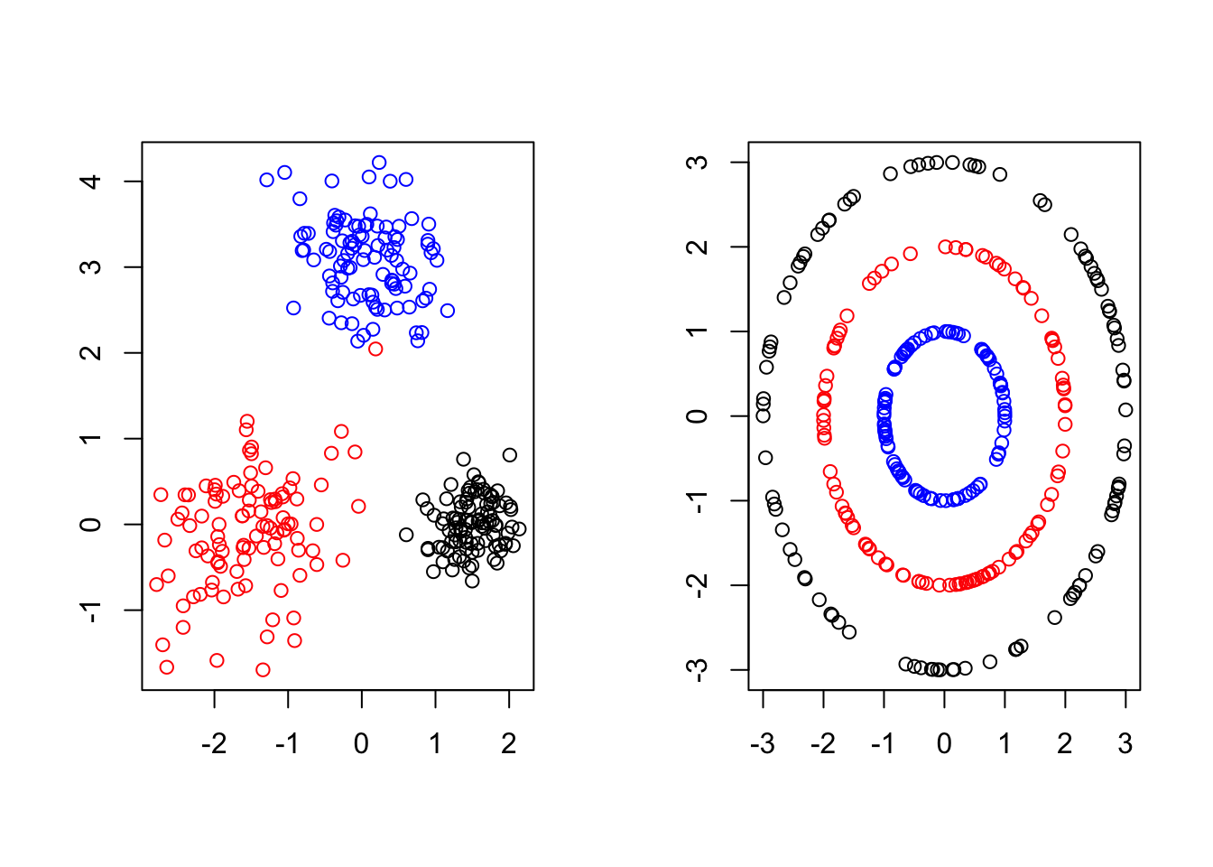
Figure 3.3: In each subfigure below, different subsets of points were generated using different rules and are colored accordingly . Ideally, a clustering algorithm could detect the different cluster shapes (left: ellipsoids, right: concentric rings) and correctly group points depending on how they were generated.
If one did not have access to the actual data generating process (depicted by the different colors), it is still likely that they could recover the correct groupings upon visual inspection. In general, this strategy is not tractable. Naturally, we would like an Unsupervised clustering algorithm that can learn these clusters directly from the data automatically. As we shall see in Chapter 7, certain algorithms will excel at grouping the data contained in disjoint ellipsoids will naturally struggle data clustering in concentric rings because the shape(s) of the different clusters matters has a major impact of the accuracy of the clustering.
In both examples above a two step sampling procedure was used to generate the observations in different clusters. First, a latent cluster label was generated. Then based on that label, an associated data point was created. Below we show an example which generates data in one of two spirals. For sample \(i\), we first draw \(z_i\sim Ber(1/2)\). Then if \(z_i=0\), we randomly generate \(x_i\) in the first spiral, otherwise we generate \(x_i\) in the second.
Example 3.4 (Intertwined spirals)
# define functions for different spirals
spiral1 <- function(u){c(u*cos(3*u),u*sin(3*u))}
spiral2 <- function(u){c(u*cos(3*(u+pi)),u*sin(3*(u+pi)))}
# sample latent cluster assignments
z <- sample(c(0,1),size = 1e3,prob = c(1/2,1/2),replace = T)

# generate spirals based on labels
X <- matrix(NA,nrow = N,ncol = 2)
for (i in 1:N){
  if (z[i]==0)
    X[i,] <- spiral1(runif(1,0.5,3))
  else
    X[i,] <- spiral2(runif(1,0.5,3))
}
#plot
plot(X, col = c("blue","red")[z+1], xlab =expression(x[1]),ylab =expression(x[2]))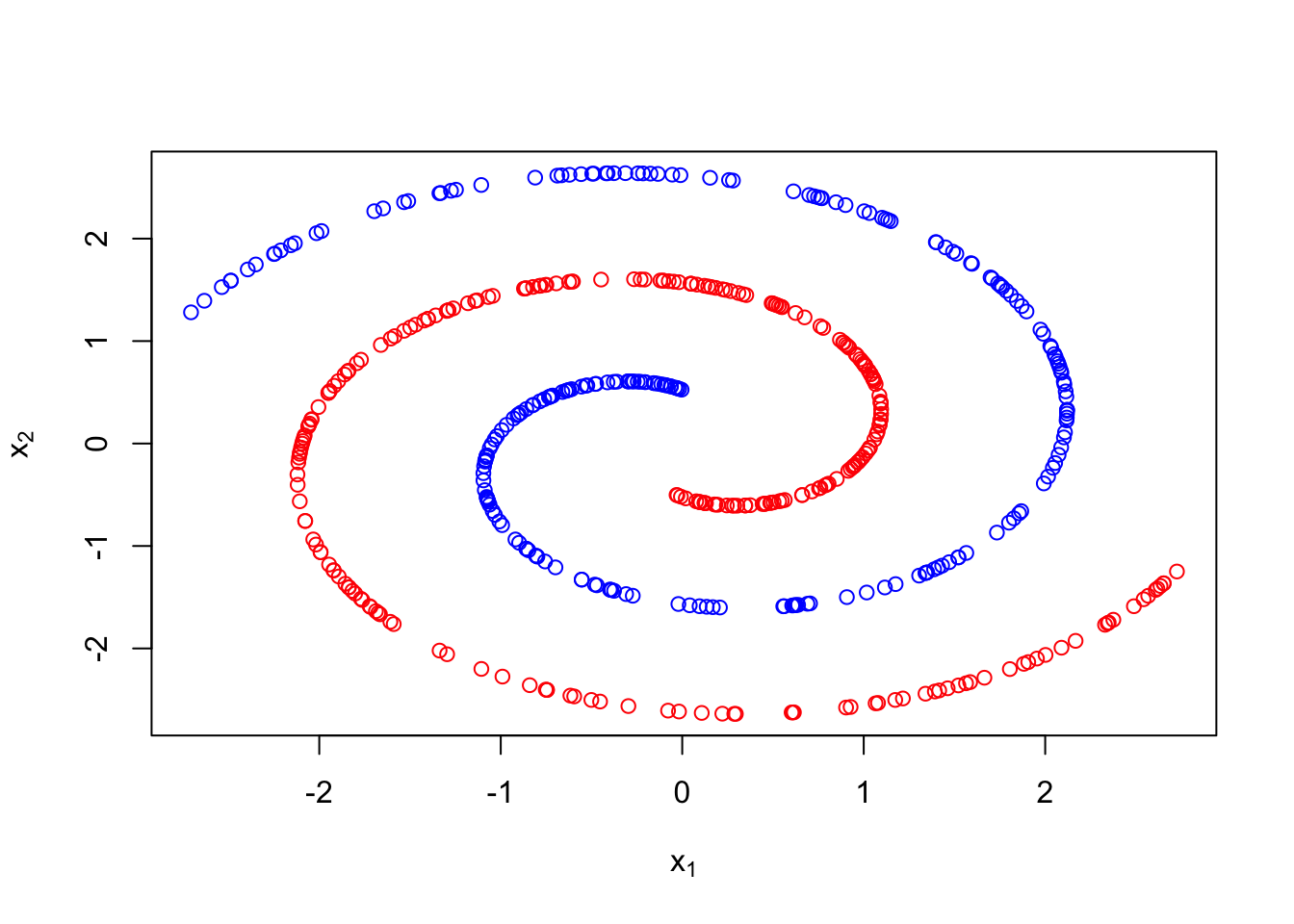
3.4 Exercises
Generate data on a helix in \(\mathbb{R}^3\).
Generate data on a 7 dimensional hyperplane in \(\mathbb{R}^{50}\). No columns of the associated data matrix should contain all zeros.
Generate 2 well separated spherical clusters in \(\mathbb{R}^3\). What is the Euclidean distance between the two closest points in different clusters?
Repeat problem 4 for \(\mathbb{R}^{10}\) and \(\mathbb{R}^{100}\). What changes did you have to make to keep the clusters well separated (at least as far apart as problem 3)?