Chapter 6 Manifold Learning

6.1 The Manifold Hypothesis

In Chapter 4, we focused our attention on linear manifolds and saw cases where this structure was insufficient. Using kernel PCA, we tried to find a workaround by first (implicity) mapping our data to a higher dimensional feature space then approximating results with linear subspaces (of feature space). In this Chapter, we will investigate several methods to estimate a lower-dimensional representation assuming the data live on a manifold, which we hereafter refer to as the manifold hypothesis. This hypothesis is the central assumptions of modern nonlinear dimension reduction methods and can be stated as follows.

Definition 6.1 (Manifold Hypothesis) The observed data \(\vec{x}_1,\dots,\vec{x}_N\in\mathbb{R}\) are concentrated on or near a manifold of intrinsic dimension \(t\ll d.\)

In the following sections, we will provide more background on the mathematical foundation of nonlinear manifolds. Specifically, what is a manifold (and what is not) and what do we mean by intrinsic dimensionality. We’ll also touch on important properties which guides the assumptions used by various methods of nonlinear dimension reduction. For now, let’s discuss a simple mechanism for generating data on a manifold.

Assume there are points \(\vec{z}_1,\dots,\vec{z}_N\in A \subset \mathbb{R}^t\) which are iid random samples from some probability distribution. These points are (nonlinearly) mapped into a higher dimensional space \(\mathbb{R}^d\) by a smooth map \(\Psi\) giving data \(\vec{x}_i = \Psi(\vec{z}_i)\) for \(i=1,\dots,N.\) Hereafter, we refer to \(\Psi\) as the manifold map. In this setting, we are only given \(\vec{x}_1,\dots,\vec{x}_N\), and we want to recover the lower-dimensional \(\vec{z}_1,\dots,\vec{z}_N\). If possible, we would also like recover \(\Psi\) and \(\Psi^{-1}\) and in the most ideal case, the sampling distribution that generated the lower-dimensional coordinates \(\vec{z}_1,\dots,\vec{z}_N\).

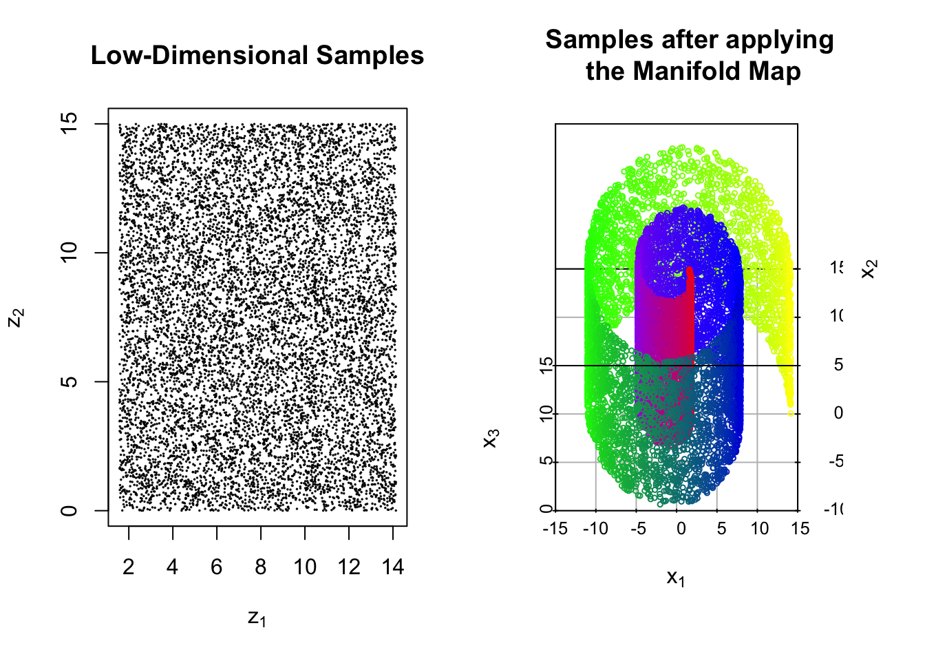
Example 6.1 (Mapping to the Swiss Roll) Let \(A = (\pi/2,9\pi/2)\times (0,15)\). We define the map \(\Psi:A\to \mathbb{R}^3\) as follows \[\Psi(\vec{z}) = \Psi(z_1,z_2) = \begin{bmatrix} z_1\sin(z_1) \\ z_1\cos(z_1) \\ z_2 \end{bmatrix}\] Below we show \(N=10^4\) samples which are drawn uniformly from \(A\). We then show the resulting observations after applying map \(\Psi\) to each sample.

We may also consider the more complicated case where the observations are corrupted by additive noise. In this setting, the typical assumption is that the noise follows after the manifold map so that our data are \[\vec{x}_i = \Psi(\vec{z}_i) + \vec{\epsilon}_i, \qquad i = 1,\dots, N\] for some noise vectors \(\{\vec{\epsilon}_i\}_{i=1,\dots,N}.\)

Example 6.2 (Swiss Roll with Additive Gaussian Noise) Here, we perturb the observations in the preceding example with additive \(\mathcal{N}(\vec{0},0.1{\bf I})\) noise.

In addition to the goals in the noiseless case, we may also add the goal of learning the noiseless version of the data which reside on a manifold.

However, there are a number of practical issues to this setup. First, the dimension, \(t\), of the original lower-dimensional points is typically unknown. Similar to previous methods, we could pick a value of \(t\) with the goal of visualization, base our choice off of prior knowledge, or run our algorithms different choices of \(t\) and compare the results. More advanced methods for estimating the true value of \(k\) are an open area of research [20].

There is also a issue with the uniqueness problem statement. Given only the high dimensional observations, there is no way we could identify the original lower-dimensional points without more information. In fact, one could find an unlimited sources of equally suitable results.

Let \(\Phi:\mathbb{R}^t\to\mathbb{R}^t\) be an invertible function. As an example, you could think of \(\Phi\) as defining a translation, reflection, rotation, or some composition of these operations akin to the nonuniqueness issue we addressed in classical scaling. If our original observed data are \(\vec{x}_i = \Psi(\vec{z}_i)\), our manifold learning algorithm could instead infer that the manifold map is \(\Psi \circ \Phi^{-1}\) and the lower-dimensional points are \(\Phi(\vec{z}_i)\). This is a perfectly reasonable result since \((\Psi\circ \Phi^{-1})\circ\Phi(\vec{z}_i) = \Psi(\vec{z}_i)= \vec{x}_i\) for \(i=1,\dots,N\), which is the only result we require. Without additional information, there is little we could do to address this issue. For the purposes of visualization, however, we will typically be most interested in the relationship between the lower-dimensional points rather than their specific location or orientation. As such, we need not be concerned about a manifold learning algorithm that provides a translated or rotated representation of \(\vec{z}_1,\dots,\vec{z}_N.\) More complicated transformations of the lower-dimensional coordinates are of greater concern and may be addressed through additional assumptions about the manifold map \(\Psi.\)

In the following sections, we will review a small collection of different methods which address the manifold learning problem. Many of the methods are motivated based on important concepts from differential geometry, the branch of mathematics focused on manifolds. Many of the details of differential geometry are beyond the scope of this book, so we will focus on a few key ideas here. For the more mathematically-minded reader, see [21, 22].

6.2 Brief primer on manifolds

While our data may exhibit some low-dimensional structure, there is no practical reason to expect such behavior to be inherently linear. In the resulting sections, we will explore methods which consider nonlinear structure and assume the data reside on or near a manifold. Such methods are referred to as nonlinear dimension reduction or manifold learning. Critical to this discussion is the notion of a manifold.

Definition 6.2 (Informal Definition of a Manifold) A manifold is a (topological) space which locally resembles Euclidean space. Each point on a \(t\)-dimensional manifold has a neighborhood that can be mapped continuously to \(\mathbb{R}^t\). We call \(t\) the intrinsic dimension of the manifold.

We’ll return to mathematical details shortly, but let’s stick with intuition for now. If you were to stand at any point on a \(k\)-dimensional manifold, the portion of the manifold closest to you look just like a \(k\)-dimensional hyperplane – though you might need to be extremely near-sighted for this to be true. The canonical example is the surface of the Earth. If we take all points on the surface of the Earth, they form a sphere in \(\mathbb{R}^3\). However, if we focus on the area around any point it looks like a portion of the two-dimensional plane. In fact, we can represent any point on the surface of the Earth in terms of two numbers, latitude and longitude. In the language of manifolds, we can say the surface of the Earth is a manifold with intrinsic dimension two which has been embedded in \(\mathbb{R}^3\). Here are a few more concrete examples.

Example 6.3 (Examples of Manifolds) Many familiar geometric objects are manifolds such as lines, planes, and spheres. For example, Let \(\vec{w}_1,\dots,\vec{w}_k\in\mathbb{R}^d\) be a set of linearly independent vectors. Then \(\text{span}(\vec{w}_1,\dots,\vec{w}_k)\) is a \(k\)-dimensional manifold in \(\mathbb{R}^d.\) When \(k=1\), the span is a line; for \(k>1\) the span is a hyperplane. The sphere unit sphere \(\{\vec{x}\in\mathbb{R}^d:\,\|\vec{x}\|=1\}\) is a \(d-1\) dimensional manifold. For example, when \(d=3\) manifold resembles the surface of the earth which locally looks like a portion of the 2-dimensional plane. The swiss roll example above is a two-dimensional manifold in \(\mathbb{R}^3\).

In short manifold as a nice smooth, curved surface. There are several reasons why a subset may not be a manifold. The most straightforward examples are cases where the manifold as a self intersection or a sharp point.

Example 6.4 (Non-manifold) Consider a figure eight curve. At the midpoint where the upper and lower circle meet, there is not neighborhood that resembles Euclidean space so the surface is not a manifold.

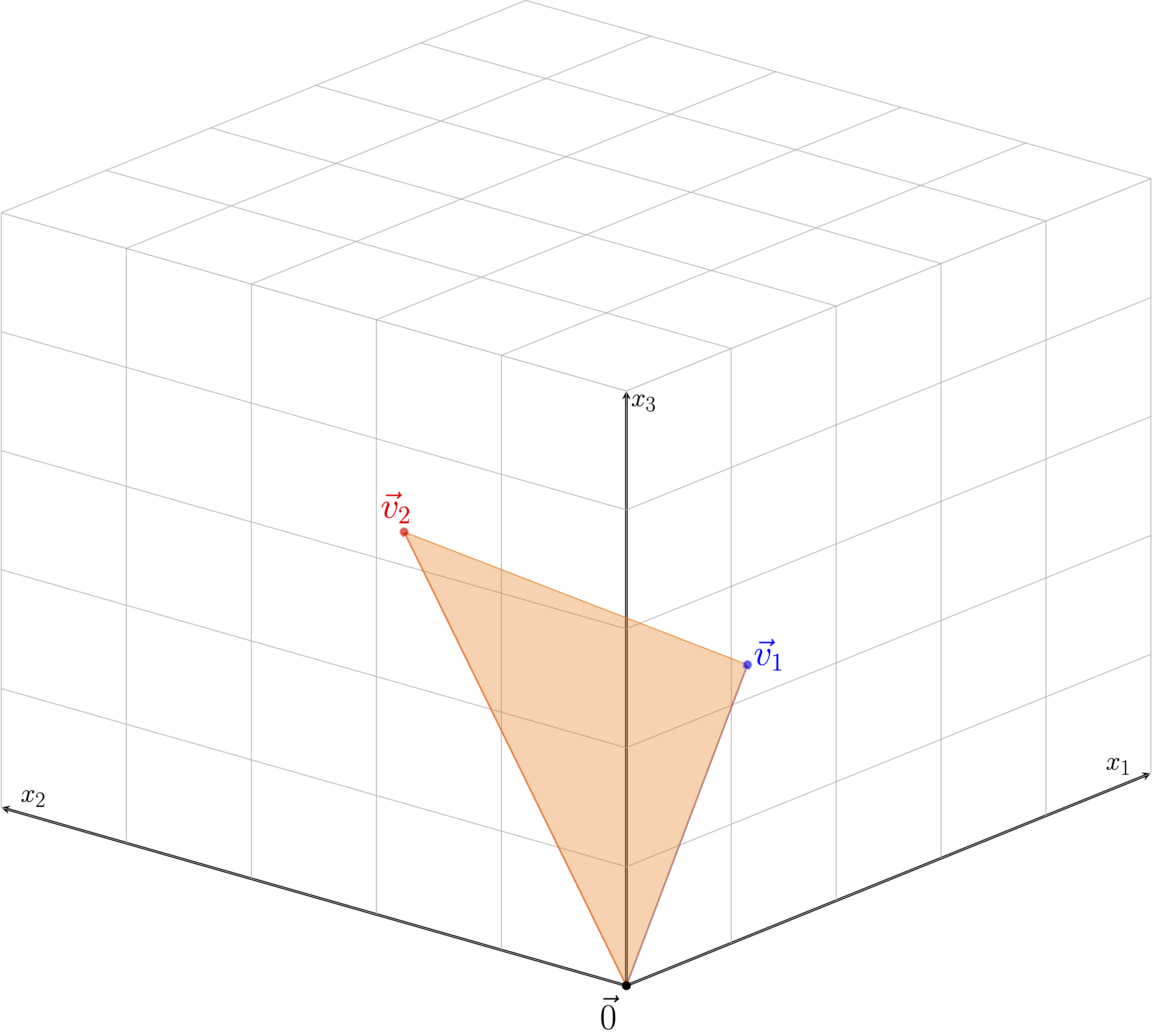
For a second example, take any two vectors \(\vec{h}_1\) and \(\vec{h}_2\) and consider there convex hull, that is \(\{a\vec{h}_1+b\vec{h}_2: a,b > 0, a+b\le 1\}\) such the orange triangle in the figure below. At the three vertices of the orange triangle, there is no local neighbor that looks flat. However, if we were to exclude the edges and vertices of the triangle, the subset would be a two-dimensional manifold; thus, \(\{a\vec{h}_1+b\vec{h}_2: a,b > 0, a+b< 1\}\) is a manifold while \(\{a\vec{h}_1+b\vec{h}_2: a,b > 0, a+b\le 1\}\) is not.

6.2.1 Charts, atlases, tangent spaces and approximating tangent planes

Hereafter, we will focus on manifolds which are a subset of \(\mathbb{R}^d\), which are often referred to as submanifolds. Differential geometry can be made far more abstract, but that is unnecessary for the discussion here. After all, we’re dealing with finite dimensional data so any nonlinear surface containing our data must be a submanifold of \(\mathbb{R}^d\)!

Now, some mathematical foundation. Let \(\mathcal{M}\) be a manifold in \(\mathbb{R}^d\) with intrinsic dimension \(t<d\). For every point \(\vec{x}\in\mathcal{M}\), there is a neighborhood \(U_x\subset \mathcal{M}\) containing \(\vec{x}\) and a function \(\phi_x: U_x \to \phi_x(U_x) \subset \mathbb{R}^t\) which is continuous, bijective, and has continuous inverse (a homeomorphism if you like greek). The pair \((U_x,\phi_x)\) is called a chart and behaves much like a map of the area around \(\vec{x}\). There are many choices for \(\phi_x\), but we can always choose one which maps \(\vec{x}\in\mathbb{R}^d\) to the origin in \(\mathbb{R}^t\). For vectors \(\vec{z}\in U_x\), we call \(\phi_x(\vec{z})\in\mathbb{R}^t\) the local coordinates of \(\vec{z}.\)

Example 6.5 (Charts and Manifold Maps) Let’s revisit the swiss roll example from the previous section where \(A = (\pi/2,9\pi/2)\times (0,15)\). We defined the map \(\Psi:A\to \mathbb{R}^3\) as follows \[\Psi(\vec{z}) = \Psi(z_1,z_2) = \begin{bmatrix} z_1\sin(z_1) \\ z_1\cos(z_1) \\ z_2 \end{bmatrix}.\] For other manifolds, we may need multiple charts to cover the manifold, but we only need one chart the swiss roll (or any manifold defined through a homeomorphic manifold map). Let the neighborhood be the entire manifold, i.e. \(U = \mathcal{M}\) Given \(\vec{x}=(x_1,x_2,x_3)^T\), let \(\phi(\vec{x}) = (\sqrt(x_1^2+x_2^2),x_3)^T.\) This chart essentially unrolls the swiss roll and turns it back into a rectangle in \(\mathbb{R}^2\) so that the local coordinates are the original coordinates!

If we take a collection of charts \(\{U_x,\phi_x\}_{x \in \mathcal{I}}\) such that \(\cup_{x\in\mathcal{I}}U_i = \mathcal{M}\), we have at atlas for the manifold. Here \(\mathcal{I}\) is a subset of \(\mathcal{M}\) which could be countable or finite. With a chart, we can consider doing differential calculus on the manifold. In particular, if \(f:\mathcal{M}\to\mathbb{R}\), then for a chart \((U_x,\phi_x)\), the function \(f\circ \phi_x^{-1}\) is a map from a subset of \(\mathbb{R}^t\) (namely \(\phi_x(U)\)) to \(\mathbb{R}\) so we might hope that we could apply the typical rules of calculus. However, if we have two charts \((U_y,\phi_y)\) and \((U_x,\phi_x)\) which overlap – \((U_x\cap U_y) \ne \emptyset\) – then derivatives \(f\circ \phi_x^{-1}\) and \(f\circ \phi_y^{-1}\) should agree on \(U_x\cap U_y\). More succinctly, the rules of calculus should remain consistent across charts!

Definition 6.3 (Differentiable Manifolds) An atlas \(\{U_x,\phi_x\}_{x\in\mathcal{M}}\) is differentiable if the transition maps \(\phi_x \circ \phi_y^{-1}: \phi_y(U_y) \to \mathbb{R}^t\) are differentiable functions. Recall \(\phi_y(U_y)\subset\mathbb{R}^t\) so differentiable in this case follows the traditional Euclidean definition from calculus.

With some additional properties and manifold with a differential atlas is a differentiable manifold allowing us to compute derivatives of function from the manifold to the reals. We’ll revisit this detail again when discussion Hessian Local Linear Embeddings. For now, let’s assume we have a differentiable manifold with intrinsic dimension \(t\). To every point on the manifold, we can attach a \(t\)-dimensional tangent space. There are several methods for defining the tangent space, but the most straightforward involves the case where we have a manifold map. We’ll restrict our attention to this case.

Definition 6.4 (Tangent Space) Let \(A\subset\mathbb{R}^t\) and let \(\Psi:A\to \mathcal{M}\subset \mathbb{R}^d\). Furthermore, suppose \(\Psi\) has coordinate functions \(\Psi_1,\dots,\Psi_d: A \to \mathbb{R}\) such that for \(\vec{y}=(y_1,\dots,y_t)^T\in A\), \(\Psi(\vec{y}) = (\Psi_1(\vec{y}),\dots,\Psi_d(\vec{y}))^T.\) The Jacobian of \(\Psi\), denoted \({\bf J}_{\Psi}\) is the \(d\times t\) dimensional matrix of partial derivative such that \[({\bf J}_{\Psi})_{ij} = \frac{\partial \Psi_i}{\partial y_j}.\] The tangent space of the manifold \(\mathcal{M}\) at the point \(\vec{p}=\Psi(\vec{y})\), denoted \(T_p(\mathcal{M})\) is the column span of \(({\bf J}_{\Psi})\) evaluated at \(\vec{y}\).

The manifold locally resembles \(\mathbb{R}^t\) so the tangent space should also be \(t\)-dimensional. As such, we’ll require \({\bf J}_{\Psi}\) to be a full rank matrix (with rank \(t\) since \(t < d\)) for every \(\vec{y}\in A\). Importantly, the tangent space is a linear subspace meaning it passes through the origin. This should not be confused with tangent plane to the manifold which we now define.

Definition 6.5 (Tangent Plane) Suppose a manifold \(\mathcal{M}\) has tangent space \(T_p(\mathcal{M})\). Then the approximating tangent plane to the manifold is the affine subspace obtained by translations, namely \(\{\vec{x}\in\mathbb{R}^d: \vec{x}-\vec{p} \in T_p(\mathcal{M})\}.\)

Let’s return to the swiss roll to make these details explicit.

Example 6.6 (Jacobians and Tangent Space for the Swiss Roll) The Jacobian of the swiss roll map is \[{\bf J}_{\Psi} = \begin{bmatrix} z_1\cos(z_1) + \sin(z_1) & 0 \\ -z_1\sin(z_1) + \cos(z_1) & 0 \\ 0 & 1 \end{bmatrix}.\] At the point \(\Psi(3\pi/2,5)=(-3\pi/2,0,5)^T\) the Jacobian is \[{\bf J}_{\Psi}\mid_{(3\pi/2,5)^T} = \begin{bmatrix} -1 & 0 \\ -3\pi/2 & 0 \\ 0 & 1 \end{bmatrix}\] so \[T_{(3\pi/2,0,5)^T}(\mathcal{M}) = \text{span}\{(1,3\pi/2,0)^T, (0,0,1)^T\}.\] We can view the associated approximating tangent plane (translucent blue) at the point \((3\pi/2,0,5)^T\) (in red).

6.2.1.1 Estimating properties from data

In the preceding subsection, we needed to manifold map to define charts, local coordinates, and tangent spaces. However, we do not have access to the manifold map only samples we assume are living near or on an \(t\)-dimensional manifold. In fact, we do not typically know \(t\) either. Fortunately, ideas we have discussed previously can allow us to estimate intrinsic dimensionality, local coordinates, and tangent spaces from data. The key idea is to zoom in on a sufficiently small neighborhood of the manifold that looks inherently Euclidean.

Suppose we have sample \(\vec{x}_1,\dots,\vec{x}_N\in\mathcal{M}\). Given a point \(\vec{x}\in\mathcal{M}\) – typically a sample in our data set – we can first find \(k\) nearest points to \(\vec{x}\) using Euclidean distance. Without loss of generality, let’s call them \(\vec{x}_1,\dots,\vec{x}_k\). If the nearest neighbors are sufficiently close to \(\vec{x}\) they should reside close to a \(t\)-dimensional hyperplane! We can then apply PCA to \(\vec{x}_1,\dots,\vec{x}_k\) or SVD to the displacements \(\vec{x}_1-\vec{x},\dots,\vec{x}_k-\vec{x}\). We expect to see a sharp drop after \(t\) eigenvalues (or singular values) allowing us to estimate the intrinsic dimension \(t\). Subsequently, the first \(t\) PCA scores (or first \(t\) columns of \({\bf US}\) in the SVD) serve as local coordinates for \(\vec{x}_1,\dots,\vec{x}_k\). Finally, the first \(t\) PC loadings (or first \(t\) right singular vectors) are an approximate basis for the tangent space.

Example 6.7 (Estimating Local Properties from Samples) Suppose we are given \(N=10^4\) samples from the Swiss roll. Let’s see how the SVD appraoch outlined above performs at estimating the tangent space at \(\Psi(3\pi/2,5) = (-3\pi/2,0,5)^T=\vec{x}.\) As an example, we’ll plot the singular values of the SVD of the data matrix with rows \(\vec{x}_1^T-\vec{x}^T,\dots, \vec{x}_k^T-\vec{x}^T\). We’ll investigate for a range of \(k\).

The sharp drop after \(t=2\) is striking for \(k >5\) nearest neighbors. Furthermore, this method does an excellent job at estimating the tangent space. Below, we show the associated approximating hyperplane which we estimate using the first two right singular vectors of the data matrix using the first 15 neighbors. The results look visually indiscernible from the case where the Jacobian was used.

SVD and PCA still have their uses thanks to the locally Euclidean nature of manifolds. Naturally, the quality of the estimations depends on having sufficiently dense sampling on the manifold. Verifying results are robust to \(k\) is a good place to start, but this approach has been formalized into a more reliable method for estimating the intrinsic dimensionality of a manifold[23].

6.3 Isometric Feature Map (ISOMAP)

6.3.1 Introduction

The first manifold learning method we are going to cover is the Isometric Feature Map (ISOMAP), originally published by Tenenbaum, de Silva, and Langford in 2000 [24]. As suggested by the name, we will see that the assumption of isometry is central to this method. ISOMAP combines the major algorithmic features of PCA and MDS — computational efficiency, global optimality, and asymptotic convergence guarantees. Thanks to these extraordinary features, ISOMAP is capable of learning a broad class of nonlinear manifolds.

6.3.2 Key Definitions

Different notions of pointwise distance

Prior to discussing the ISOMAP algorithm, let’s briefly discuss the notion of isometry through an example which motivates different notions of distance between two points.

Example 6.8 (Distance between points on a Helix) Consider the helix map \(\Psi:\mathbb{R}\to\mathbb{R}^3\) given by the formula \[\begin{equation} \Psi(t) = \begin{bmatrix} \frac{1}{\sqrt{2}}\cos(t) \\ \frac{1}{\sqrt{2}}\sin(t) \\ \frac{1}{\sqrt{2}}t \\ \end{bmatrix} \end{equation}\] Below, we show the result of applying the Helix map to each point in the interval \((0,25)\). Let’s focus on two points \(\vec{x}_1 = \Psi(2\pi)= (1/\sqrt{2},0,\sqrt{2}\pi)^T\) and \(\vec{x}_2 = \Psi(4\pi)=(1/\sqrt{2},0,2\sqrt{2}\pi)^T\) in particular which are shown as large black dots in the figure below.

There are a few different ways we could measure the distance between the two black points. The first approach would be to ignore the helix (manifold) structure viewing them as vectors in \(\mathbb{R}^3\) and directly measure their Euclidean distance which gives \[\|\vec{x}_1 - \vec{x}_2\| = \sqrt{2}\pi.\] However, we also know that these points are images of the one-dimensional coordinate \(z_1 = 2\pi\) and \(z_2 = 4\pi\) respectively. Thus, we could also consider the Euclidean distance of the lower-dimemsional coordinates which is \(|2\pi - 4\pi| = 2\pi\), which notably differs from the Euclidean distance.

A third option is to return to the three-dimensional representation but to also account for the manifold structure when considering distance. Recall Euclidean distance gives the length of the shortest, straightline path connecting the two points. Instead, let’s restrict ourselves to only those paths which stay on the helix (manifold). You may correctly conclude that the curve starting at \(\Psi(2\pi)\), rotating up the helix one rotation, and ending at \(\Psi(4\pi)\) is the shortest such path. Fortunately, computing arc-length is relatively friendly in this example since \(\Psi\) already parameterizes the path connecting these two points. The arc-length is then \[\int_{2\pi}^{4\pi} \left\|\frac{d\Psi}{dt}\right\| dt = \int_{2\pi}^{4\pi} dt = 2\pi.\] Jumping slightly ahead, we then say the manifold distance between \(\Psi(2\pi)\) and \(\Psi(4\pi)\) is \(2\pi\). Importantly, the manifold distance coincides exactly with the Euclidean distance between the lower-dimensional coordinates. In fact, for any two points, \(s\) and \(t\), on the real line their Euclidean distance, \(|s-t|\) will be the same as the manifold distance between \(\Psi(s)\) and \(\Psi(t)\). Thus, the helix map \(\Psi\) above serves as our first example of an isometric (distance preserving) map.

We may generalize this idea to any smooth manifold to define a new notion of distance. Given a manifold \(\mathcal{M}\), we define the manifold distance function \(d_{\mathcal{M}} : \mathcal{M} \times \mathcal{M} \to [0,\infty)\) as follows

Definition of Manifold Distance ::: {.definition #def-manifold-dist name=“Manifold Distance Function”} Given two points \(\vec{x}\) and \(\vec{y}\) on a smooth manifold, \(\mathcal{M}\), let \(\Gamma(\vec{x},\vec{y})\) be the set of all piecewise smooth curves connecting \(\vec{x}\) and \(\vec{y}\) constrained to stay on \(\mathcal{M}\). Then, we define the manifold distance to be \[\begin{equation} d_{\mathcal{M}}(\vec{x},\vec{y}) = \inf_{\gamma \in \Gamma(\vec{x},\vec{y})} L(\gamma) \tag{6.1} \end{equation}\] where \(L(\gamma)\) is the arclength of \(\gamma.\)
:::

As we reviewed above, the helix example with the arclength formula is one example of a manifold and distance function. Additional examples of a manifold and manifold distance include,

• Euclidean space \(\mathbb{R}^d\) where standard Euclidean distance gives the manifold distance.
• The sphere in \(\mathbb{R}^3\) which is a two-dimensional manifold. Its manifold distance is also called the Great Circle Distance.

We may now define the notion of isometry which is a central assumption of ISOMAP.

Definition of Isometry ::: {.definition #def-isometry name=“Isometry”} Let \(\mathcal{M}_1\) be a manifold with distance function \(d_{\mathcal{M}_1}\) and let \(\mathcal{M}_2\) be a second manifold with distance function \(d_{\mathcal{M}_2}\). The mapping \(\Psi:\mathcal{M}_1 \mapsto \mathcal{M}_2\) is an isometry if \[d_{\mathcal{M}_1}(x,y) = d_{\mathcal{M}_2}\left(\Psi(\vec{x}),\Psi(\vec{y})\right) \qquad \text{ for all } \vec{x},\vec{y}\in \mathcal{M}_1.\] :::

For the purposes of ISOMAP, we will think of \(\mathcal{M}_1\) as some subset of a \(\mathbb{R}^k\) for \(k\) small where we measure distances using the Euclidean norm. Then \(\mathcal{M}_2\) will be a \(k\)-dimensional manifold in \(\mathbb{R}^d\) containing our data. Our first assumption is that the manifold mapping \(\Psi\) is an isometry. Unfortunately, in practice we do not know the manifold nor will we have a method for parameterizing curves on the manifold to compute distances.

6.3.3 Algorithm

Instead, ISOMAP makes use of a data-driven approach to estimate the manifold distance between points following a three-step procedure.

1) Construct Weighted Neighborhood Graph:

MDS uses Euclidean distance to measure pairwise distance between points \(\vec{x}_i\) and \(\vec{x}_j\) (data points in space \(\mathcal{M}_2\)), while ISOMAP uses the geodesic distance in order to reveal the underlying manifold structure. However, when the data points in the high dimensional space \(\mathcal{M}_2\) have a manifold structure, usually the Euclidean pairwise distance is quite different from their pairwise geodesic distance. Fortunately, for small distances on a smoothly embedded manifold, the geodesic path between two close-by points lies nearly flat in the ambient space. So, the length of this path will be very close to the straight line (Euclidean) distance between those points in the ambient space.

The key intuition is that as the density of data points on the manifold increases (i.e., points get closer and closer), the straight line segment in the ambient space connecting two neighboring points becomes a better and better approximation of the shortest path between those points on the manifold. In the limit of the density going to infinity, these distances converge.

Let’s elucidate this concept with two illustrative examples. Firstly, imagine a two-dimensional surface, like a Swiss Roll, situated within a three-dimensional space. For an ant journeying across the Swiss Roll, the vast size difference means its immediate surroundings appear flat. From its perspective, the distance between its consecutive steps closely mirrors the distance a human might measure (Euclidean distance) – both virtually equating to the roll’s geodesic distance. For a larger-scale analogy, think of Earth. Suppose extraterrestrial beings possessed technology allowing them to traverse straight through Earth’s crust and mantle, thus following the shortest Euclidean path. Their journey from Los Angeles to New York might save them hundreds of miles compared to humans. However, when moving between closer landmarks, such as the Science Center to the Smith Center, their advantage diminishes.

As a result, when it comes to the measurement of geodesic distance, it is reasonable to only look at those data points that are close to each other. First, calculate all the pairwise Euclidean distance \(d_{ij}=||\vec{x}_i - \vec{x}_j||_2\), then determine which points are neighbors on the manifold by connecting each point to Either (i) All points that lie within a ball of radius \(\epsilon\) of that point; OR (ii) all points which are K-nearest neighbors with it. (Two different criteria, \(K\) and \(\epsilon\) are tuning parameters)

According to this rule, a weighted neighborhood graph \(G = G(V,E)\) can be built. The set of vertices (data points in space \(\mathcal{M}_2\)): \(V = \{\vec{x}_1, \dots , \vec{x}_N\}\) are the input data points, and the set of edges \(E = \{e_{ij}\}\) indicate neighborhood relationships between the points. \(e_{ij} = d_{ij}\) if (i) \(||\vec{x}_i - \vec{x}_j||_2 \leq \epsilon\); OR (ii) \(\vec{x}_j\) is one of the K-nearest neighbors of \(\vec{x}_i\), otherwise \(e_{ij} = \infty\). Sometimes, the tuning of \(\epsilon\) (or \(K\)) is quite decisive in the output of ISOMAP, we will explain this later with a simulation example.

2) Compute graph distances

In this step, we want to estimate the unknown true geodesic distances \(\{d^{\mathcal{M}}_{ij}\}\) between all pairs of points with the help of the neighborhood graph \(G\) we have just built. We use the graph distances \(\{d^{\mathcal{G}}_{ij}\}\)— the shortest distances between all pairs of points in the graph \(G\) to estimate \(\{d^{\mathcal{M}}_{ij}\}\). For \(\vec{x}_i\) and \(\vec{x}_j\) that are not connected to each other, we try to find the shortest path that goes along the connected points on the graph. Following this particular sequence of neighbor-to-neighbor links, the sum of all the link weights along the path is defined as \(\{d^{\mathcal{G}}_{ij}\}\). In other words, we use a number of short Euclidean distances (representing the local structure of the manifold) to approximate the geodesic distance \(\{d^{\mathcal{M}}_{ij}\}\).

This path finding step is usually done by Floyd-Warshall algorithm, which iteratively tries all transit points \(k\) and find those that \(\tilde{d}_{ik} + \tilde{d}_{kj} < \tilde{d}_{ij}\), and updates \(\tilde{d}_{ij} = \tilde{d}_{ik} + \tilde{d}_{kj}\) for all possible combination of \(i,j\). The algorithm works best in dense neighboring graph scenario, with a computational complexity of \(O(n^3)\).

The theoretical guarantee of this graph distance computation method is given by Bernstein et, al.[25] one year after they first proposed ISOMAP in their previous paper. They show that asymptotically (as \(n \rightarrow \infty\)), the estimate \(d^{\mathcal{G}}\) converges to \(d^{\mathcal{M}}\) as long as the data points are sampled from a probability distribution that is supported by the entire manifold, and the manifold itself is flat.

The distance matrix \(\Delta\) can be expressed as: \[\Delta_{ij} = d^{\mathcal{G}}_{ij}\]

Simulation Example

Here we provide a randomly generated Neighborhood Graph for six data points, it uses the K-nearest neighbor criteria (can easily tell this since the matrix is not symmetric, \(K=2\))

# Define the matrix
matrix <- matrix(c(
  0,   3,  4,   Inf, Inf, Inf,
  7,   0,  Inf, 2,   Inf, Inf,
  6,   Inf,0,   Inf, 7,   Inf,
  Inf, 5,  Inf, 0,   Inf, 10,
  Inf, Inf,8,   Inf, 0,   13,
  Inf, Inf,Inf, 9,   14,  0
), byrow = TRUE, nrow = 6)
print(matrix)

##      [,1] [,2] [,3] [,4] [,5] [,6]
## [1,]    0    3    4  Inf  Inf  Inf
## [2,]    7    0  Inf    2  Inf  Inf
## [3,]    6  Inf    0  Inf    7  Inf
## [4,]  Inf    5  Inf    0  Inf   10
## [5,]  Inf  Inf    8  Inf    0   13
## [6,]  Inf  Inf  Inf    9   14    0

Shown below is the implementation of Floyd-Warshall algorithm in R. As you can see from the three for loops, its computation complexity is \(O(n^3)\).

# Adjusting the matrix to set d_ij and d_ji to the smaller value
n <- dim(matrix)[1]

for (i in 1:n) {
  for (j in 1:n) {
    if (i != j && is.finite(matrix[i, j]) && is.finite(matrix[j, i])) {
      min_val <- min(matrix[i, j], matrix[j, i])
      matrix[i, j] <- min_val
      matrix[j, i] <- min_val
    }
  }
}

# Floyd-Warshall Algorithm
floyd_warshall <- function(mat) {
  n <- dim(mat)[1]
  dist <- mat
  
  for (k in 1:n) {
    for (i in 1:n) {
      for (j in 1:n) {
        dist[i, j] <- min(dist[i, j], dist[i, k] + dist[k, j])
      }
    }
  }
  
  return(dist)
}

# Get the result
result <- floyd_warshall(matrix)

# Print the result
print(result)

##      [,1] [,2] [,3] [,4] [,5] [,6]
## [1,]    0    3    4    5   11   14
## [2,]    3    0    7    2   14   11
## [3,]    4    7    0    9    7   18
## [4,]    5    2    9    0   16    9
## [5,]   11   14    7   16    0   13
## [6,]   14   11   18    9   13    0

3) Applying MDS to \(\Delta\)

As mentioned before, ISOMAP can be viewed as the application of classical MDS in non-linear case. As a result, the reconstruction of \(\{\vec{z}_i\}\) in the \(k\) dimensional \(\mathcal{M}_1\) follows similar steps as that of classical MDS. The main goal is to preserve the geodesic distance of the manifold in \(\mathcal{M}_2\) as much as possible.

Without any additional information, there are infinite \(\{\vec{z}_i\}\) that can be viewed as the optimal solution. For some invertible function \(\Phi:\mathbb{R}^k\to\mathbb{R}^k\), a new manifold mapping \(\Psi \circ \Phi^{-1}\) can be constructed. \(\vec{x}_i = \Psi \circ \Phi^{-1} (\Phi(\vec{z}_i))\), which proofs that \(\{\Phi(\vec{z}_i)\}\) is equivalent to \(\{\vec{z}_i\}\) when it comes to the reconstruction of the lower dimensional configuration.

Without loss of generality, we assume that \(\{\vec{z}_i\}\) are actually centered. So the distance matrix of \(\{\vec{z}_i\}\) can be expressed as \(B=Z^T Z\), so that \(B_{ii}=||z_i||^2_2\) and \(B_{ij}={z_i}^T z_j\).

The embedding vectors \(\{\hat{z}_{i}\}\) (estimate of points in lower dimensional feature space \(\mathcal{M}_1\)) are chosen in order to minimize the objective function:

\[(\sum ||\vec{z}_i - \vec{z}_j||_2 - \Delta_{ij})^2\]

Following the same procedure explained in classical MDS chapter, we can compute each entry of \(B\): \[B_{ij}= -\frac{1}{2} \Delta^2_{ij} + \frac{1}{d} \sum^{d}_{i=1} \Delta^2_{ij} + \frac{1}{d} \sum^{d}_{j=1} \Delta^2_{ij} - \frac{1}{2d^2} \sum^{d}_{i=1} \sum^{d}_{j=1} \Delta^2_{ij}\]

To express it in matrix form, it is actually, \(B = - \frac{1}{2} H \Delta H\), where \(H = I_n - \frac{1}{n} \mathbb{1} \mathbb{1}^T\).

The next step is just a PCA problem. Implement eigen decomposition on matrix B, \(B=U \Lambda U^T= (\Lambda^{1/2} U)^T (\Lambda^{1/2} U)\), then arrange the singular value in descending order, find the first \(k^{\prime}\) ones. We acquire \(\Lambda_{k^{\prime}}\) and \(U_{k^{\prime}}\). \[(\hat{z}_1 | \hat{z}_2 | \dots | \hat{z}_N) = \Lambda_{k^{\prime}} U_{k^{\prime}}\]

Since we don’t know the dimension of the underlying feature space, here \(k^{\prime}\) is a tuning parameter. Usually, we use a scree plot (\(k^{\prime}\) against the sum of the omitted eigenvalues ) and find the elbow point.

6.3.4 Limitations of ISOMAP

Though ISOMAP is a powerful manifold learning method that works well under most circumstances. It still has some limitations in certain scenarios.

1. If the noises \(\{\epsilon_i\}\) is not negligible, then ISOMAP may fail to identify the manifold. Also, ISOMAP is quite sensitive to the tuning parameters. To alleviate the negative impact, it’s highly suggested to start with a relatively small \(\epsilon\) or \(K\), and increase them gradually.

2. When data points are sparse in certain areas or directions of the manifold, the integrity of the learned manifold structure can be compromised. The following example will clarify this notion:

3. One of the two major assumptions of ISOMAP is the convexity of the manifold, that is to say, if the manifold contains many holes and concave margins, then the result of ISOMAP will probably be not ideal.

6.4 Locally Linear Embeddings (LLEs)

6.4.1 Introduction

Locally linear embedding (LLE) is an unsupervised learning algorithm first introduced in 2000 by Sam T. Roweis and Lawrence K. Saul [26]. In the original four-page paper, the two authors introduced the LLE algorithm and demonstrated its effectiveness in dimensional reduction, manifold learning, and in handling real-world high-dimensional data. Unlike clustering methods for local dimensional reduction, LLE maps its inputs into a single global coordinate system of lower dimensionality, and its optimizations do not involve local minima. By exploiting the local symmetries of linear reconstructions, LLE is able to learn the global structure of nonlinear manifolds, such as those generated by images of faces or documents of text. Thanks to its great mathematical properties and relatively low computing cost (compared to other manifold learning methods, like ISOMAP), LLE quickly became attractive to researchers after its emergence due to its ability to deal with large amounts of high dimensional data and its non-iterative way of finding the embeddings [27]. Compared to ISOMAP and some other previous manifold learning methods, LLE is computationally simpler and can give useful results on a broader range of manifolds [28].

For dimensional reduction, most methods introduced before LLE need to estimate pairwise distances between even two remote data points, no matter it is the simple Euclidean distance (classical MDS) or more sophisticated manifold distance (ISOMAP). The underlying main idea of these methods is actually finding a configuration that recovers all pairwise distances of original data points as much as possible. LLE, however, is quite different from these previous methods as it focuses on preserving locally linear relationships.

6.4.2 Algorithm

LLE algorithm is actually built on very simple geometric intuitions. As explained in MDS Part, if we consider a small enough region on a manifold in \(D\) dimensional space, in most cases, it can be regarded as a \(d\) dimensional hyperplane (\(d \ll D\)). LLE also makes use of this intuition and assumes that the whole manifold consist of numerous \(d\)-dimensional patches that have been stitched together. Assuming that there exists sufficient data (data points are compact), it is reasonable to expect that each data point and its neighbors lie on or close to a locally linear patch of the manifold.

Following this idea, LLE approximates each data point by a weighted linear combination of its neighbors and proceeds to find a lower-dimensional configuration of data points so that the linear approximations of all data points are best preserved.

Specifically speaking, LLE algorithm consists of three steps. The initial step involves selecting a certain number of each data point’s nearest neighbors based on Euclidean distance. Following this, the second step calculates the optimal reconstruction weights for each point using its nearest neighbors. The final step carries out the embedding while maintaining the local geometry depicted by the reconstruction weights.

6.4.2.1 Construct Neighborhood Graph

This step is actually very similar to that of ISOMAP. The process of finding neighbors in LLE is typically conducted using grouping methods like k-nearest neighbors (KNN) or selecting neighbors within a fixed radius ball (\(\epsilon\)-neighborhoods), based on the Euclidean distance for each data point, in the provided data set. The KNN method is predominantly utilized for its straightforwardness and ease of implementation. The following explanations are based on KNN method.

Denote \(N\) data points in original \(D\) dimensional space as \(\vec{x}_1, \vec{x}_2, \dots, \vec{x}_N \in \mathbb{R}^D\). For a point \(\vec{x}_i, \quad 1 \leq i \leq N\), its neighbor set is defined as \(N_i^k \subseteq \{1, 2, 3, \dots, i-1, i+1, \dots, N \}\), where \(N_i^k\) can also be called as the indices of \(k\) nearest neighbors of \(\vec{x}_i\). The tuning parameter \(k\) is chosen small enough so that the patch around \(\vec{x}_i\) is flat. However, \(k\) should also be strictly larger than \(d\) so as to let the algorithm work.

As we can tell from these, LLE works well only if data points are dense and hopefully evenly distributed, which will be explained in detail in later examples. The parameter tuning of the appropriate number of neighbors, \(k\), faces challenges of complexity, non-linearity, and diversity of high-dimensional input samples. A larger \(k\) value might cause the algorithm to overlook or even lose the local nonlinear features on the manifold. This issue is exacerbated as neighbor selection, typically based on Euclidean distance, can result in distant neighbors when considering the intrinsic geometry of the data, akin to a short circuit. Conversely, an overly small \(k\) value may lead the LLE algorithm to fragment the continuous manifold into isolated local pieces, losing global characteristics.

6.4.2.2 Reconsruct with Linear Weights

As put before, we try to reconstruct each \(\vec{x}_i\) using an almost convex weighted combination of its neighbors. The respective weights of all its neighbors \(\vec{x}_j, \; j \neq i\) for each \(\vec{x}_i\) is quite essential in the later reconstruction of the underlying intrinsic configuration, as we consider these weights to remain invariant before and after mapping.

To explain it in mathematical formulas, the approximate of \(\vec{x}_i\): \(\tilde{x}_i\) is defined as \(\tilde{x}_i = \sum_{j=1}^N w_{ij} \vec{x}_j\). There are two constraints for this formula: First, \(w_{ij} \equiv 0\), if \(j \notin N_i^k\) (consistent with the assumption of \(k\) nearest neighbors); Second, the sum of weights for each \(\vec{x}_i\) is always zero, i.e., \(\sum_{j=1}^N w_{ij}=1\).

Then, the problem of finding the optimal \(w_{ij}, \; 1 \leq i,j \leq N\) is equivalent to solving the following constrained Least Squares problem for \(\forall 1 \leq i \leq N\):

(1) \[ \begin{aligned} & \min \left\| \vec{x}_i-\sum_{j \in N_i^k} w_{i j} \vec{x}_j\right\|^2 \\ & \text { s.t. } \quad \sum_{j \in N_i^k} w_{i j}=1 . \end{aligned} \]

It is worth noting that the weights can be negative theoretically, though in practice, we don’t expect that to happen.

Invariance to Rotation, Rescaling and Transaction

Define \(\epsilon(w) = \sum_{i=1}^N \left\| \vec{x}_i-\sum_{j \in N_i^k} w_{i j} \vec{x}_j\right\|^2\), which is the cost function.

1. \(\epsilon(w)\) is unchanged by rotation or rescaling by common factor

Actually \(\sum_{i=1}^N \left\| a \text{U} \vec{x}_i-\sum_{j \in N_i^k} w_{i j} a \text{U} \vec{x}_j\right\|^2 = a^2 \epsilon(w)\), where \(a\) is a non-zero scaler and \(\text{U}\) is an orthonormal matrix.

2. \(\epsilon(w)\) is unchanged by transactions

Thanks to the constraint that \(\sum_{j=1}^N w_{ij}=1\), for any transaction \(\vec{x}_i \rightarrow \vec{x}_i + \vec{y}\), the cost function does not change.

\[\sum_{i=1}^N \left\| (\vec{x}_i + \vec{y}) -\sum_{j \in N_i^k} w_{i j} (\vec{x}_j + \vec{y}) \right\|^2 = \sum_{i=1}^N \left\| \vec{x}_i-\sum_{j \in N_i^k} w_{i j} \vec{x}_j\right\|^2 = \epsilon(w)\]

From the expressions, we develop a strategy that optimizes one row of matrix \(w\) at a time. Now let’s try to rewrite \(\epsilon(\vec{w}_i)=\left\| \vec{x}_i-\sum_{j \in N_i^k} w_{i j} \vec{x}_j\right\|^2\).

\[\begin{align} \epsilon(\vec{w}_i) &= \left\| \vec{x}_i-\sum_{j \in N_i^k} w_{i j} \vec{x}_j\right\|^2 \\ & = \left[ \sum_{j=1}^N w_{ij} (\vec{x}_i - \vec{w}_j) \right]^T \left[ \sum_{l=1}^N w_{il} (\vec{x}_i - \vec{w}_l) \right]^T \\ & = \sum_{j=1}^N \sum_{l=1}^N w_{ij} w_{il} (\vec{x}_i -\vec{x}_j)^T (\vec{x}_i - \vec{x}_l) \\ & = \vec{w}_i^T G_i \vec{w}_i \end{align}\]

\(\vec{w}_i^T = (w_{i1}, w_{i2}, \dots w_{iN})\) is the \(i^{th}\) row of W. Here \(G_i \in \mathbb{R}^{N \times N}\), where entry \(G_{i}(j.l), \; 1 \leq j,l \leq N\) can be represented as:

\[ G_{i}(j,l) = \begin{cases} (\vec{x}_i - \vec{x}_j)^T (\vec{x}_i - \vec{x}_l) & j,l \in N_i^k \\ 0 & j \; or \; l \notin N_i^k \end{cases} \]

The \((j,l)\) entry of \(G_i\) is actually the inner product of \(\vec{x}_j\) and \(\vec{x}_l\) when centered around \(\vec{x}_i\). From this expression, we know that actually \(G_i\) is a sparse matrix and can be reduced to a compact matrix \(\tilde{G}_i \in \mathbb{R}^{k \times k}\) that eliminates those empty columns and rows.

\[\begin{align} \tilde{G}_i & = (\vec{x}_{i[1]} - \vec{x}_i, \dots, \vec{x}_{i[k]} - \vec{x}_i)^T (\vec{x}_{i[1]} - \vec{x}_i, \dots, \vec{x}_{i[k]} - \vec{x}_i) \\ & = Q_i^T Q_i \end{align}\]

where \([1]\) denotes the first entry in \(N_i^k\). So \(\tilde{G}_i\) is actually a real symmetric and positive semi-definite matrix.

Now let’s go back to deal with the optimization function — Equation 1 can be solved with Lagrange multiplier given that it has only equality constraints. (More details about the use of Lagrange multiplier can be found in [Lagrange multiplier]https://en.wikipedia.org/wiki/Lagrange_multiplier)

Optimizing Equation 1 is equivalent to minimizing (for \(\forall 1 \leq i \leq N\)) \[ f(\vec{w}_i, \lambda) = \vec{w}^T_i G_i \vec{w}_i - \lambda (\vec{w}^T_i \mathbf{1}_k -1) \] which has the result: \[ \vec{w}_i^{\star} = \frac{\tilde{G}^{-}_i \mathbf{1}_k}{\mathbf{1}^T_k \tilde{G}^{-}_i \mathbf{1}_k} \]

Complement:

As discussed before, we can only proof that \(\tilde{G}_i\) is positive semi-definite, however, we cannot ensure that it is positive definite, which means \(\tilde{G}_i\) is not necessarily invertible. That is why we use the generalize inverse sign here. In practice, it can be done through performing SVD on \(\tilde{G}_i\) and select the first few large singular values and eliminate the rest. Then when computing \(\tilde{G}^{-}_i\), just do the reciprocal of these retained singular values.

Actually \(\tilde{G}_i\) only has \(d\) (the intrinsic original dimension if you forget) relatively large eigenvalues. The rest are either very small or zeros. So it is very likely that \(\tilde{G}_i\) is singular, making the computation result highly unstable. In {[28]}, the authors proposed to address this issue through regularizing \(\tilde{G}_i\).

\[ \tilde{G}_i \leftarrow \tilde{G}_i+ \left(\frac{\Delta^2}{k}\right) \operatorname{Tr}\left(\tilde{G}_i\right) \mathbf{I} \] Here \(Tr(\tilde{G}_i)\) denotes the trace of \(\tilde{G}_i\) and \(\Delta \ll 1\).

6.4.2.3 Embedding

In the previous step, we have recovered the optimal weight matrix

\[ \mathbf{W} = \left(\begin{array}{l} \vec{w}_1^T \\ \vdots \\ \vec{w}_N^T \end{array}\right) \]

The optimal weights \(\mathbb{W}\) reflects local, linear geometry around each \(\vec{x}_i\), thus if the configuration \(\vec{y}_1, \vec{y}_2, \dots, \vec{y}_N \in \mathbb{R}^d\) are the lower dimensional representation, they should also “match” the local geometry.

Following this idea, the objective function is:

(2) \[ \begin{aligned} & \underset{\mathbf{Y}}{\text{argmin}} \sum_{i=1}^N \left\| \vec{y}_i - \sum_{j=1}^{N} w_{ij} \vec{y}_j^T \right\|^2 \\ = & \underset{\mathbf{Y}}{\text{argmin}} \sum_{i=1}^N \left\| \sum_{j=1}^N w_{ij} (\vec{y}_i - \vec{y}_j)^T \right\|^2 \\ = & \underset{\mathbf{Y}}{\text{argmin}} \left\| \mathbf{Y - WY} \right\|_F^2 \\ = & \underset{\mathbf{Y}}{\text{argmin}} \left\| (\mathbf{I}_N - \mathbf{W}) \mathbf{Y} \right\|_F^2 \\ = & \underset{\mathbf{Y}}{\text{argmin}} \; \text{Tr} \left[ \mathbf{Y}^T (\mathbf{I}_N - \mathbf{W})^T (\mathbf{I}_N - \mathbf{W}) \mathbf{Y} \right] \end{aligned} \] where \(\mathbf{Y}=(\vec{y}_1 | \vec{y}_2 | \dots | \vec{y}_N)^T\)

There are two constraints:

1. \(\mathbf{1}_N^T \mathbf{Y} = \vec{0}\). This forces \(\vec{y}\) to be centered

2. \(\frac{1}{N} \mathbf{Y}^T \mathbf{Y} = \mathbf{I}_d\). This fixes rotation and scaling.

Key Observation

Considering the final expression of Equation 2, the optimization function is now equivalent to finding \(\vec{y}_i\)s that minimizes \(\mathbf{Y}^T (\mathbf{I}_N - \mathbf{W})^T (\mathbf{I}_N - \mathbf{W}) \mathbf{Y}\).

Here we introduce \(\mathbf{M} = (\mathbf{I}_N - \mathbf{W})^T (\mathbf{I}_N - \mathbf{W})\), which is a positive semi-definite matrix. Since \(\mathbf{M} \mathbf{1}_N = (\mathbf{I} - \mathbf{W})^T (\mathbf{1}_N - \mathbf{W} \mathbf{1}_N) = \vec{0}\), \(\mathbf{1}_N\) is an eigen-vector of \(\mathbf{M}\) with eigenvalue zero.

\[ \begin{aligned} \mathbf{Y}^T (\mathbf{I}_N - \mathbf{W})^T (\mathbf{I}_N - \mathbf{W}) \mathbf{Y} = \mathbf{Y}^T \mathbf{M} \mathbf{Y} \end{aligned} \] From constraint (b), we know that columns of \(\mathbf{Y}\) are orthogonal to each other. As a result, this whole problem can be simplified to finding the eigen-vectors of \(\mathbf{M}\) with the smallest eigenvalues.

Compute eigen-vectors with the smallest \(d+1\) eigenvalues \(0=\lambda_1 \leq \lambda_2 < \dots < \lambda_{d+1}\), eliminate \(\mathbf{1}_N\) (the first one). The remaining \(d\) vectors are respectively \(\vec{v}_2, \vec{v}_3, \dots \vec{v}_{d+1} \in \mathbb{R}^N\). So \(\mathbf{Y} = (\vec{v}_2 | \vec{v}_2 | \dots | \vec{v}_{d+1})\), we successfully recover the corresponding \(\vec{y}_1, \vec{y}_2, \dots, \vec{y}_N \in \mathbb{R}^d\).

An illustration of the algorithm

In the original paper [26], the authors provide a very intuitive plot that summarizes the above three steps.

LLE_illustration

Parameter Tuning

There are two parameters to tune in LLE, i.e. (the number of neighbors: \(k \,\); the dimension of the recovered configuration: \(d \,\)).

1. For selection of \(d\), we usually use a reverse scree plot and find the elbow point. It is worth noting that we are choosing the smallest \(d+1\) eigenvalues and compute their corresponding eigen-vectors here. Since the eigen-vectors and eigenvalues of a particular matrix is super sensitive to any sort of noises or perturbations, especially for those small eigenvalues, it is hard to accurately derive the corresponding eigen-vectors \(\vec{v}_2, \dots, \vec{v}_{d+1}\). This is called ill-conditioned eigen-problem.

2. Choose the optimal \(k\)

LLE seeks to preserve local structure through nearest neighbor connections. This is the key point to LLE. As a result, we may use the neighbor set of the original \(\vec{x}_1, \vec{x}_2, \dots, \vec{x}_N \in \mathbb{R}^D\) and \(\vec{y}_1, \vec{y}_2, \dots, \vec{y}_N \in \mathbb{R}^d\) as a criteria.

As explained before, we use \(N_i^k\) to denote the indices of k-nearest neighbors to \(\vec{x}_i\). Similarly, we can also use \(V_i^k\) to denote the indices of k-nearest neighbors to \(\vec{y}_i\). They should be as close as possible.

So our objective function here is: \[ Q(k)= \frac{\sum_{i=1}^N \left| N_i^k \cap V_i^k \right|}{Nk} \] Plot \(Q(k)\) against \(k\), select \(k^{\star}\) where the increase of \(Q(k)\) becomes negligible.

6.4.3 Strengths and Weaknesses of LLE

6.4.3.1 Strengths

1. High Computation Efficiency

The low computation cost of LLE algorithm may be its most shinning advantage over other manifold learning methods, and it is actually one of its biggest selling point when it was first introduced. The LLE algorithm Involves solving a sparse eigen problem, with computational complexity of roughly \(O(N^2 d^2 + N d^3)\) where \(N\) is the number of data points and \(d\) is the dimension of the recovered configuration.

In comparison, ISOMAP requires computing shortest paths between all pairs of points, which is typically done using Dijkstra’s or Floyd-Warshall algorithm, leading to a complexity of \(O(N^2 log N)\) or \(O(N^3)\) respectively. Then, it involves eigen decomposition similar to classical MDS which is \(O(N^3)\).

In practice, \(d \ll N\), hence the computation cost of LLE is lower than that of ISOMAP in most cases.

2. Few parameters to tune

There are only two parameters to tune, respectively the number of neighbors included in the map: \(k\), and the dimensional of the original configuration: \(d\). In addition, there exist clear methods to find the optimal \(k\) and \(d\), as stated in the previous part. This makes LLE algorithm easy to find the optimal parameters.

6.4.3.2 Weaknesses

1. Sensitivity to tuning parameters

The result of LLE is quite sensitive to its two control parameters: the number of neighbors \(k \,\) and the dimensional of the original configuration: \(d\).

Here we use the Swiss Roll example to illustrate this. LLE is optimal at \(k=45\). However, when \(k=40\), the recovered lower-dimensional configuration is wrong (Green points and yellow points overlap, which is not the case in Swiss Roll); and when we slightly increase \(k\) to 50, the recovered two-dimensional expression is not necessarily a rectangle.

2. Vulnerable to sparse or unevenly-distributed samples

The vulnerability towards sparsity and uneven distribution exists in almost all manifold learning methods, including ISOMAP, as we have illustrated in the previous section. LLE is not immune to this either. When a data set is unevenly distributed, since LLE relies on the original Euclidean distance metric, it tends to select neighbors from a singular direction where these neighbors are densely clustered. Clearly, using these selected neighbors to reconstruct the reference point results in significant redundancy in that specific direction. Concurrently, essential information from other directions or regions is not retained for the reconstruction of the reference point. As a result, these selected neighbors are inadequate for accurately representing and reconstructing the reference point. Consequently, much of the intrinsic structure and internal features will be lost after dimension reduction using LLE.

3. Sensitivity to noise

LLE is extremely sensitive to noise. Even a small noise would cause failure in deriving low dimensional configurations. Justin Wang, et.al utilize various visualization examples to illustrate this drawback in their paper [29], you may take a look if you are interested. Various algorithms have been developed to address this issue, i.e., Robustly Locally Linear Embedding (RLLE) [30], and Locally Linear Embedding with Additive Noise (LLEAN) [29]. The former works well when outliers exist, while the latter has a satisfactory performance when the original points are distorted with noises.

6.5 Laplacian Eigenmap

The Laplacian eigenmap [31] is method of manifold learning with algorithmic and geometric similarities to LLEs. Like LLEs and ISOMAP, Laplacian eigenmaps make use of \(k\)-nearest neighbor relationships and the solution of an eigenvalue problem to reconstruct the low-dimensional manifold. As suggested by the name, we will be using the graph Laplacian matrix and emphasize the preservation of nearby points on the manifold making Laplacian Eigenmaps a local method with a different emphasis than LLEs.

The graph Laplacian is an important matrix representation of our data which we will revisit later when discussing spectral clustering. In practice, Laplacian eigenmaps use sparse version of the graph Laplacian. For now, we will briefly introduce this matrix without sparsity and an important identity relating the graph Laplacian and the loss function we will minimize when constructing our low-dimensional representation.

Given data \(\vec{x}_1,\dots,\vec{x}_N\), we are going to build a weighted graph \(\mathcal{G}=(V,\mathcal{E}, {\bf W})\), with one node per sample and weighted, undirected edges connecting the nodes. The weights, \({\bf W}_{ij}\ge 0, \, 1\le i,j\le N\), correspond to a notion of affinity, which is typically a decreasing function of the distance between our data. Two common choices are (i) binary weights: \[{\bf W}_{ij} = \begin{cases} 1 & \|\vec{x}_i-\vec{x}_j\| \le \epsilon \\ 0 & \text{ else} \end{cases}\] and (ii) weights based on the radial basis function: \[{\bf W}_{ij} = \exp\left(-\frac{\|\vec{x}_i-\vec{x}_j\|^2}{2\sigma^2}\right). \] The symmetric matrix \({\bf W}\) is called the (weighted) adjacency matrix of the graph, \(\mathcal{G}\), encodes of all the pairwise relationships. We always set the diagonal entries of \({\bf W}\) to zero to preclude self-connections in the graph.

From the adjacency matrix, we can compute the total affinity of each node (sample) to all other nodes (samples) by summing along the rows. Specifically, the \(i\)th entry of the vector \({\bf W}\vec{1}_N\), has the total affinity of the \(i\)th node (\(\vec{x}_i\)) to all other nodes (data). Using these summed affinities, we then create the graph Laplacian \[\begin{equation} {\bf L} = {\bf D} - {\bf W} \end{equation}\] where \({\bf D}\) is a diagonal matrix with entries \({\bf W}\vec{1}_N\) along its diagonal. The graph Laplacian is a symmetric matrix, and while not obvious at first glance, it is also positive semidefinite thanks to the following important identity. Given any vector \(\vec{y}\in\mathbb{R}^N\), \[\begin{equation} \vec{y}^T{\bf L} \vec{y} = \frac{1}{2} \sum_{i=1}^n\sum_{j=1}^N {\bf W}_{ij} (y_i-y_j)^2 \tag{6.2} \end{equation}\] However, it is not full rank. The previous equation shows that \(\vec{1}\) is an eigenvector with eigenvalue 0.

In the previous statement we can view the entries of vector \(\vec{y}\) as \(N\) separate scalars. However, we can also extend the preceding expression to include Euclidean distances between vectors \(\vec{y}_1,\dots,\vec{y}_N\in\mathbb{R}^t\) to give the following important expression \[\begin{equation} \sum_{i=1}^N\sum_{j=1}^N {\bf W}_{ij} \|\vec{y}_i-\vec{y}_j\|^2 = \frac{1}{2}tr\left({\bf Y}^T{\bf LY}\right) \end{equation}\] where \({\bf Y}\in\mathbb{R}^{N\times t}\) has rows \(\vec{y}_1^T,\dots,\vec{y}_N^T.\) We will return to this identity and its implications for Laplacian Eigenmaps after discussing the algorithmic details of the method

6.5.1 Algorithm

6.5.1.1 Compute neighbor relationships

Fix either a number of nearest neighbors \(k > 0\) or maximum distance \(\epsilon > 0\). If using \(\epsilon\), then \(\vec{x}_i\) and \(\vec{x}_j\) (correspondingly nodes \(i\) and \(j\) in the graph) are neighbors if \(\|\vec{x}_i-\vec{x}_j\| \le \epsilon\). Alternatively, if using the nearest neighbor parameter \(k\), then we consider \(\vec{x}_i,\vec{x}_j\) to be neighbors if \(\vec{x}_i\) is one the \(k\) closest points to \(\vec{x}_j\) and \(\vec{x}_j\) is one of the \(k\) closest points to \(\vec{x}_i.\) The construction of neighbors, like the use of pairwise distance alone, results in symmetric neighbor relationship. We then connect nodes \(i\) and \(j\) with an edge if \(\vec{x}_i\) and \(\vec{x}_j\) are neighbors.

6.5.1.2 Compute weights and build graph Laplacian

Nodes which are not connected immediately receive an edge weight equal to zero. For all connected nodes, we compute the edge weight \[{\bf W}_{ij} = \exp\left(-\frac{\|\vec{x}_i-\vec{x}_j\|^2}{2\sigma^2}\right).\] Here we have shown weights based on the radial basis function, which is motivated by theoretical connections to the heat kernel and an approximation of the Laplacian on the manifold \(\mathcal{X}\) [31]. As such, this method is the default in most implementation of Laplacian eigenmaps. The parameter \(\sigma^2\) does require tuning which can have a large impact on the performance of the algorithm.

When \(k\) or \(\epsilon\) are small, which is typically the case in practice, the (weighted) adjacency matrix \({\bf W}\) will be sparse (most entries equal to 0). From this adjacency matrix, we then construct the graph Laplacian as above. The graph Laplacian built from these weights will also be sparse. By preserving only those connections between nearest points, we have only maintained the pairwise, local relationships on the manifold. We will now use \({\bf L}\) to construct a lower-dimensional representation of the data.

6.5.1.3 Solve generalized eigenvalue problem

Consider the loss function \[\begin{equation} \mathcal{L}(\vec{y}_1,\dots,\vec{y}_N) = \sum_{i=1}^N\sum_{j=1}^N {\bf W}_{ij} \|\vec{y}_i-\vec{y}_j\|^2. \end{equation}\] This loss function is most sensitive to large pairwise distance \(\|\vec{y}_i-\vec{y}_j\|\) when \({\bf W}_{ij}\) is also large (our original data were close). Thus, minimizing the preceding penalty prioritizes keeping \(\vec{y}_i\) and \(\vec{y}_j\) close when \(\vec{x}_i\) and \(\vec{x}_j\) have a high affinity (weight). As a result, Laplacian eigenmaps emphasize local geometry.

Vectors \(\vec{y}_1,\dots,\vec{y}_N\) which minimizes this loss function are not unique. First, there is an issue of translation. To address this issue, we will add a constraint that \({\bf D Y}\) is a centered data matrix, i.e. \({\bf Y}^T{\bf D}\vec{1} = \vec{0}\). We can view the matrix \({\bf DY}\) as a reweighting of the data matrix \({\bf Y}\) with higher weights \({\bf D}_{ii}\) for data \(\vec{x}_i\) which are closer to more points. Here \({\bf D}\) is the diagonal matrix used in the definition of the graph Laplacian. Note that \[{\bf DY} = \begin{bmatrix} {\bf D}_{11} \vec{y}_1^T \\ \vdots \\ {\bf D}_{NN}\vec{y}_N\end{bmatrix}.\] Requiring \({\bf DY}\) to be centered results in configurations where those points with highest affinity a constrained close to the origin in our lower dimensional representation.

However, solving the optimization problem with this modified centering constraint is still ill-posed, namely we could take \(\vec{y}_1=\dots=\vec{y}_N = \vec{0}\) giving a configuration which is collapsed onto the origin. In fact, given any configuration \(\vec{y}_1,\dots,\vec{y}_N\) we could decrease the loss by rescaling all of our data by some constant scalar scalar \(0 < c < 1\) since \({\bf D}(c{\bf Y}) = c {\bf DY}\) will still be centered. To address this scaling issue and give a meaningful \(t\)-dimensional configuration, we also add the constraint \({\bf Y}^T {\bf D Y} = {\bf I}_t\). This constraint eliminates the collapse of the \(t\)-dimensional configuration onto a \(t-1\) dimensional hyperplane, and in particular eliminates the cases where the \(1-\)dimensional configuration collapses onto a point.

Thus, we seek a data matrix \({\bf Y}\in\mathbb{R}^{N\times t}\) solving the following constrained optimization problem \[\begin{equation} \text{argmin}_{{\bf Y}^T {\bf D Y} = {\bf I}_t, {\bf Y}^T{\bf D}\vec{1}^T = \vec{0} } = tr({\bf Y}^T {\bf L Y}). \end{equation}\] To solve this problem, we first introduce the change of variable \(\tilde{\bf Y} = {\bf D}^{1/2}{\bf Y}\) so that the constraints become \[{\bf Y}^T{\bf D}\vec{1}^T = ({\bf D}^{1/2} {\bf Y})^T{\bf D}^{1/2}\vec{1}^T = \tilde{\bf Y}^T {\bf D}^{1/2} \vec{1}^T = \vec{0}\] and
\[{\bf Y}^T{\bf D Y}= {\bf Y}^T{\bf D}^{1/2} {\bf D}^{1/2}{\bf Y} = ({\bf D}^{1/2}{\bf Y})^T ({\bf D}^{1/2}{\bf Y}) = \tilde{\bf Y}^T\tilde{\bf Y} = {\bf I}\] implying that the columns of \(\tilde{\bf Y}\) are orthonormal After the change of variable, our optimization problem becomes \[\begin{equation} \text{argmin}_{\tilde{\bf Y}^T\tilde{\bf Y} = {\bf I}_t, \tilde{\bf Y}^{1/2} {\bf D}^{1/2}\vec{1} = \vec{0} } tr\left(\tilde{\bf Y}^T {\bf D}^{-1/2}{\bf L}{\bf D}^{-1/2}\tilde{\bf Y} \right). \end{equation}\] We can minimize this equation by making use of the eigenvalues and eigenvectors of the (symmetric) normalized graph Laplacian \[{\bf L}_{sym} = {\bf I} - {\bf D}^{-1/2}{\bf W}{\bf D}^{-1/2}.\]

Importantly, note that \({\bf L}_{sym}\) is symmetric. Furthemore, it is positive semidefinite since it can be viewed as the graph Laplacian of a graph with weights \({\bf W}_{ij}/\sqrt{{\bf D}_{ii}{\bf D}_{jj}}\) thus subject to the identity (6.2). Thus, it is diagonalizable with orthonormal eigenvectors \(\vec{v}_1,\dots,\vec{v}_N\in\mathbb{R}^N\) and associated nonnegative eigenvalues \(\lambda_1 \le \dots \le \lambda_N\) which we list in increasing order in this case. This leads to the first important observation

1. We could use any \(t\) of these vectors as the columns of \(\tilde{Y}\) and immediately satisfy the constraint \(\tilde{\bf Y}^T\tilde{\bf Y} = {\bf I}.\)

However, we have an additional constraint and the minimization to consider. Note that \(\vec{1}_N\) is an eigenvector of original graph Laplacian with eigenvalue \(0\). Thus, \({\bf L}_{sym}\) also has eigenvalue 0 with associated eigenvector \(\vec{v}_1 = {\bf D}^{1/2}\vec{1}\) since \[{\bf L}_{sym} ({\bf D}^{1/2}\vec{1}) ={\bf D}^{-1/2}({\bf D}^{1/2} - {\bf W D}^{-1/2}){\bf D}^{1/2}\vec{1} = {\bf D}^{-1/2}({\bf D}-{\bf W})\vec{1} = {\bf D}^{-1/2} {\bf L}\vec{1} = \vec{0}.\] As a result, all other eigenvectors of \({\bf L}_{sym}\) must be orthogonal to \(\vec{v}_1 = {\bf D}^{1/2}\vec{1}.\)

2. This suggests that if we drop the first eigenvector associated with eigenvalue \(\lambda_1 = 0\) and use \(t\) the remaining eigenvectors of \({\bf L}_{sym}\) as the columns of \(\tilde{\bf Y}\) we will satisfy the constraint \(\tilde{\bf Y}^T {\bf D}^{1/2}\vec{1} = \vec{0}.\)

The finaly observation is that we should choose the eigenvectors to minimize the objective.

3. We make use of the eigenvalues themselves and take \[\tilde{Y} = \begin{bmatrix} \vec{v}_2 & \dots & \vec{v}_{t+1} \end{bmatrix}\] so that \[tr\left( \tilde{\bf Y}^T{\bf L}_{sym}\tilde{\bf Y}\right) = \lambda_2+\dots+\lambda_{t+1}\] is minimized.

After undoing the change of variables, we take use the rows of \[{\bf Y} = {\bf D}^{-1/2}\tilde{\bf Y}\in \mathbb{R}^{N\times t}\] as our \(t\)-dimensional configuration.

6.6 Hessian Eigenmaps (HLLEs)

6.6.1 Introduction

To motivate Hessian eigenmaps, let us revisit the revisit the idea of derivatives on real valued functions on the manifold. Suppose we have a manifold \(\mathcal{M} \subset \mathbb{R}^d\) and function \(f:\mathcal{M}\to\mathbb{R}\). Assuming that \(\mathcal{M}\) has intrinsic dimension \(t < d\), to each point \(\vec{x}\in\mathcal{M}\), we can associate a \(t\) dimensional tangent space \(T_{\vec{x}}(\mathcal{M})\) which we equip with a choice of orthonormal basis vectors. Furthermore, there is an open neighborhood \(U\) containing \(\vec{x}\) with every point in the neighborhood in one to one correspondence with a point in the tangent space allowing us to conduct calculus on the manifold using approximations within the tangent space.

Theorem 6.1 (Null Space of Hessian Operator on Manifolds) Suppose \(\mathcal{M} = \Psi(\Theta)\) where \(\Theta\) is an open, connected subset of \(\mathbb{R}^t\), and \(\Psi\) is a locally isometric embedding of \(\Theta\) into \(\mathbb{R}^d\). Then \(\mathcal{H}(f)\) has a \(t+1\) dimensional null space spanned by the constant function and a \(t\)-dimensional space of functions spanned by the original isometric coordinates.

Suppose now that we have a function \(f:\mathcal{M}\to \mathbb{R} \subset\mathbb{R}^d\) and we wish to estimate \(\mathcal{H}(f)\) using observed data \(\vec{x}_1,\dots,\vec{x}_N\in\mathcal{M}\). HLLEs are based around the construction of a discretized estimation of \(\mathcal{H}(f)\) which we can write in the quadratic form \[\vec{f}^T{\bf H}\vec{f} \text{ where } \vec{f} = \left(f(\vec{x}_1),\dots,f(\vec{x}_N)\right)^T\in\mathbb{R}^N.\] The matrix \({\bf H}\in\mathbb{R}^{N\times N}\) is symmetric and positive semidefinite and depends only on the observed data \(\vec{x}_1,\dots,\vec{x}_N\). Its construction will be discussed in greater detail in the algorithms section below.

For now, assume that we have access to \({\bf H}\). Suppose that \(f\) is in the null space of \(\mathcal{H}(f)\) then i) \(\vec{f}^T{\bf H}\vec{f} \approx 0\) and ii) from Theorem ?? it must be the case that \(f(\vec{x}_i) = \alpha + \beta^T\vec{z}_i\). Importantly, if we can identify the null space of the matrix \({\bf H}\) then we can use this to recover the original low-dimensional coordinates (up to rigid motion and coordinate rescaling).

Similar to LLEs and ISOMAP, this algorithm begins with a k-nearest neighbor search and finishes with a eigenvalue decomposition. As inputs we provide the data, the intrinsic dimension, \(t\), of the manifold, and a specified number of nearest neighbors \(k\). For reasons we’ll discuss later, we must select \(k > t(t+3)/2\). This constraint can be problematic in practice. For example, if we believe the intrinsic dimension of \(\mathcal{M}\) is 100, then we need to pick \(k > 5150\) meaning we need at least 5151 samples in our dataset! Such a constraint may be difficult to satisfy in practice, but for dimension reduction focused on visualization with the ambition assumption that \(t=1,2,\) or \(3\), \(k \ge 10\) is sufficient.

6.6.1.1 Compute nearest neighbors and local coordinates

For each \(\vec{x}_i\) compute its \(k\)-nearest neighbors which we’ll denote \(\mathcal{N}_i\). We’ll use each of these neighbors to estimate the Hessian of \(f\) at \(\vec{x}_i\). Next we’ll estimate local coordinates of the neighbors in \(\mathcal{N}_i\) by using SVD to approximate the tangent plane \(T_{\vec{x}_i}(\mathcal{M})\). One important observation to recall. We expect the points in \(\mathcal{N}_i\) to all be close together and centered around \(\vec{x}_i\). In this neighborhood around \(\vec{x}_i\) we expect the manifold \(\mathcal{M}\) to look like a small patch of \(\mathbb{R}^d\). As such, they should be (nearly) contained in a \(t\)-dimensional affine subspace of \(\mathbb{R}^d.\)

Let \({\bf M}_i \in \mathbb{R}^{k\times d}\) be the matrix of centered nearest neighbors of \(\vec{x}_i\). Specifically, the \(j\)th row of \({\bf M}_i\) is \((\vec{x}_{i_j} - \vec{x}_i)^T\) where \(\vec{x}_{i_j}\) is the \(j\)th nearest neighbor of \(\vec{x}_i\). We apply a singular value decomposition to \({\bf M}_i\) giving factorization \[{\bf M}_i = {\bf U}_i {\bf S}_i {\bf V}_i^T\] where \({\bf U}\in\mathbb{R}^{k\times k}\) abd \(V_i\in\mathbb{R}^{k\times k}\) have orthonormal columns and \({\bf S}_i\in\mathbb{R}^{k\times d}\) is diagonal. If the neighbors in \(\mathcal{N}_i\) were fully contained in a t-dimensional affine subspace we expect that \({\bf S}_i\) has \(t\) large singular values with the remainder equal to zero. Additionally in this case, the tangent space \(T_{\vec{x}_i}\) is \(\vec{x}_i + \text{span}\{\vec{v}_1,\dots,\vec{v}_t\}\) where \(\vec{v}_1,\dots,\vec{v}_t\) are the first \(t\) columns of \({\bf V}\).

In practice, we should only expect the first \(t\) singular values to be large with the remainder smaller but non-zero. However, we’ll still use the first \(t\) columns of \({\bf V}\) as an (approximate) orthonormal basis for the tangent space. The first \(t\) columns of \({\bf U}_i{\bf S}_i\) give approximations of the local coordinates of the neighbors \(\mathcal{N}_i\) in this neighborhood (the \(j\)th row gives the local coordinates for the \(j\)th nearest neighbor). Hereafter, we’ll let \(\vec{u}^i_j = (u^i_{j1},\dots,u^i_{jt})^T\) denote the local coordinates of the \(j\)th nearest neighbor in the tangent space.

6.6.1.2 Estimate the Hessian

Recall from section 6.2, that we can define derivatives for a function \(f\) at \(\vec{x}_i\) using the local coordinates.

Now, we can use the local gradients and Hessians to construct a Taylor approximation to \(f(\vec{x}_j)\) for each point in the neighbor \(\mathcal{N}_j\). In the tangent space \(T_{\vec{x}_i}(\mathcal{M})\), we associate the origin with \(\vec{x}_i\). Taylor expanding around the origin to second order we have the following approximation \[\begin{align*} f(\vec{x}_{i_j}) &\approx f(\vec{x}_i) + \left[\nabla^{tan} f(\vec{x}_i)\right]^T \cdot \vec{u}^i_j + \frac{1}{2}(\vec{u}^i_j)^T \left(H^{tan}f (\vec{x}_i)\right)\vec{u}^i_j\\ &= f(\vec{x}_i) + \sum_{\ell=1}^t \left[\nabla^{tan} f(\vec{x}_i)\right]_\ell \vec{u}^i_{j\ell} + \frac{1}{2}\sum_{\ell=1}^t \left(H^{tan}f (\vec{x}_i)\right)_{\ell\ell} (u^i_{j\ell})^2 + \sum_{\ell < s} \left(H^{tan}f (\vec{x}_i)\right)_{\ell,s} u^i_{j\ell}u^i_{js} \end{align*}\] To estimate the entries of the Hessian, we use quadratic regression. Build design matrix \({\bf X}_i \in \mathbb{R}^{k\times (1+d+d(d+1)/2)}\) including all terms up to second order of the local coordinates such that \[{\bf X}_i = \begin{bmatrix} 1 & u^i_{11} & \dots u^i_{1t} & \frac{1}{2}(u^i_{11})^2 & \dots& \frac{1}{2}(u^i_{1t})^2 & \frac{\sqrt{2}}{2}u^i_{11}u^i_{12}& \frac{\sqrt{2}}{2} u^i_{11}u^i_{13} & \dots &\frac{\sqrt{2}}{2}u^i_{1,t-1}u^i_{1t} \\ \vdots & \vdots & \vdots & \vdots & \dots & \vdots & \vdots & \vdots & \dots & \vdots\\ 1 & u^i_{k1} & \dots u^i_{kt} & \frac{1}{2}(u^i_{k1})^2 & \dots &\frac{1}{2}(u^i_{kt})^2 & \frac{\sqrt{2}}{2}u^i_{k1}u^i_{k2}& \frac{\sqrt{2}}{2}u^i_{k1}u^i_{k3} & \dots & \frac{\sqrt{2}}{2}u^i_{k,t-1}u^i_{kt} \end{bmatrix} \] If we let \(\vec{f}_i = \left(f(\vec{x}_{i_1}),\dots,f(\vec{x}_{i_k})\right)^T\) be a vector containing the function values at the nearest neighbors of \(\vec{x}_i\), then we can estimate the coefficients of the Taylor expansion using the following regression formula \[\vec{f}_i = {\bf X}^i \vec{\beta}\] where the last \(t + t(t+1)/2\) terms of \(\vec{\beta}_i\) correspond to the entries of the \(H^{tan}(f)\) at \(\vec{x}_i\). We then estimate \(\vec{\beta}_i\) using the Moore-Penrose pseudoinverse \[\vec{\beta}_i \approx ({\bf X}_i^T{\bf X})^{-1}{\bf X}_i^T \vec{f}_i.\] For the pseudoinverse to be invertible, \({\bf X}_i\) must have at least as many rows as columns. Thus, we need \(k \ge 1+t + t(t+1)/2 = 1 + t(t+3)/2 > t(t+3)/2\).

We can drop the first \(t+1\) entries which contain the intercept and the first order regression terms. Let \(\vec{\beta}_{i,drop}\) denote the final \(t(t+1)/2\) entries of \(\vec{\beta}_1\). If we square then sum the entries of \(\vec{\beta}_{i,drop}\), we now have an estimate of \(\| H^{tan}(f)\|_F^2\) at \(\vec{x}_i\).

One final note on this issue. The \(1/2\) and \({\sqrt{2}}/2\) terms in \({\bf X}_i\) are introduced to ensure we are correctly estimating (and single counting) the diagonal entries of the Hessian while double counting its upper triangular elements. This detail is missing from the original paper [32]. As such, many implementation may also replicate the mistake. Be cautious when choosing a package for implementing HLLEs!

6.6.1.3 The Eigenvalue Problem

Define \({\bf S}_i \in \mathbb{R}^{k \times N}\) as follows \[({\bf S}_i)_{j\ell} = \begin{cases} 1 & \vec{x}_\ell \text{ is the } j \text{th nearest neighbor of } \vec{x}_i \\ 0 & \text{else.} \end{cases}\] Using this notation, we can express \(\vec{f}_i\) (the function values from the k nearest neighbors of \(\vec{x}_i\)) as the product of \({\bf S}_i\) and \(\vec{f}\) (the vector containing the function value at all samples \(\vec{x}_1,\dots,\vec{x}_N\). Specifically, \(\vec{f}_i= {\bf S}_i \vec{f}\).

Now, we will use an empirical average of our Hessian estimates at each data point to approximate the operator \(\mathcal{H}(f)\) as follows \[\begin{align*} \mathcal{H}(f) &= \int_{\mathcal{M}} \|H^{tan}(f)\|_F^2 dm \\ &\approx \frac{1}{N}\sum_{i=1}^N \|\|H^{tan}\big(f\big)(\vec{x}_i)\|_F^2 \\ &\approx \frac{1}{N}\sum_{i=1}^N \|{\bf H}_i \vec{f}_i\|^2 \end{align*}\]

Now, we can make use of the identity \(\vec{f}_i={\bf S}_i \vec{f}\) to write this approximation as a quadratic function of \(\vec{f}.\) \[\begin{align*} \approx \frac{1}{N}\sum_{i=1}^N \|{\bf H}_i \vec{f}_i\|^2 &= \frac{1}{N}\sum_{i=1}^N \vec{f_i}^T{\bf H}_i^T{\bf H}_i \vec{f}_i\\ &= \frac{1}{N} \sum_{i=1}^N \vec{f}^T{\bf S}_i^T{\bf H}_i^T{\bf H}_i {\bf S}_i \vec{f} \\ &= \vec{f}^T\left(\frac{1}{N} \sum_{i=1}^N{\bf S}_i^T {\bf H}_i^T{\bf H}_i{\bf S}_i\right)\vec{f} \end{align*}\]

Letting \[{\bf H} = \frac{1}{N} \sum_{i=1}^N{\bf S}_i^T {\bf H}_i^T{\bf H}_i{\bf S}_i\] our approximation becomes \[\vec{f}^T{\bf H}\vec{f}.\] Here is the final critical observation. If \(f\) is a vector in the null space of \(\mathcal{H}\) then it must be in the span of the coordinate functions, and we would expect the approximation to be small (close to zero except for sampling variability and estimation error). As such, we can look eigenvector(s) associated with the smallest eigenvalue(s) of \({\bf H}\) to give approximations to the coordinate functions!

Like LLEs, \({\bf H}\) will have one eigenvalues which is exactly zero corresponding to the constant function. We’ll take the next \(t\) eigenvectors associated with the next smallest \(t\) eigenvalues and use them to build a data matrix. The rows of this data matrix give the corresponding low dimensional coordinates of our data.

Since \({\bf H}\) is symmetric and positive semidefinite (its is the sum of symmetric, psd matrices), its eigenvectors will be orthogonal. Selecting these eigenvectors as approximates for functions \(f_1,\dots,f_t\) giving the corresponding 1st through \(t\)th coordinates is equiavalent to imposing an orthogonality constraint on these vectors. We’ll also take the vectors to be unit length. As a result, we can expect HLLE to recover original coordinates up to rigid motion (scaling and rotation/reflection) and coordinate rescaling.

6.7 Comparison of Manifold Learning Methods

As an initial comparison, we’ll look at several 3-dimensional examples with known lower dimensional latent spaces where we can visualize the data. Importantly, these examples fail to satisfy some of the conditions of the preceding methods so we can assess how susceptible the methods we have discussed to violations in their assumptions. Table x.x summarizes the results

Table 6.1: Manifold learning examples and their properties

Manifold	Intrinsic Dimension	Preimage	Preimage connected?	Preimage convex?	Isometric Manifold Map?	Locally Isometric Manifold Map?
Helix	One	Line segment	Yes	Yes	Yes	Yes
Swiss Roll	Two	Rectangle	Yes	Yes	No	No
Folded Washer	Two	Annulus	Yes	No	No	No
Rolled Washer	Two	Annulus	Yes	No	No	No

For comparison, we provide scatterplots of 2000 samples from each manifold which we will use for analysis. The points have been color coded to improve visualization and to aid comparison with recovered lower dimensional coordinates.

6.7.1 Visual comparison of results

6.7.1.1 Helix

The helix is the simplest example and satisfies all assumptions we have discussed in the preceding sections. As such, it is not surprising that each of the methods discussed does a reasonable job compressing the data to a line segment. For the helix, we have used the isometric manifold mapping \[\Psi(t) = \left(\frac{\sqrt{2}}{2}\cos (t), \frac{\sqrt{2}}{2}\sin t, \frac{\sqrt{2}}{2} t\right)^T\] where \(t \in [0,15]\) is the original 1-dimensional coordinate for the data. Below we plot the recovered 1-d representation of the data against the corresponding value of \(t\). As we have discussed, a perfect recovery of the original \(t\) is impossible. The best we can hope for is a affine relationship reflecting a one-to-one correspondence (up to translation, rescaling, and rigid motion) between the original low dimension coordinates and those recovered by our manifold learning methods.

(#fig:helix_examples)Recovered latent space vs original coordinates

6.7.1.2 Swiss Roll

For the Swiss roll, we use the manifold map \[\Psi: \left[\frac{3\pi}{2},\frac{9\pi}{2}\right] \times [0,15] \to \mathbb{R}^3\] given by the equation \[\Psi(s,t) = \left(s\cos s, t, s\sin s\right)^T.\] Below, we plot the first and second coordinates recovered by Isomap using \(k=35\) nearest neighbors.

(#fig:swiss_examples)Recovered latent space vs original coordinates

6.7.1.3 Folded Washer

(#fig:fold_washer_examples)Recovered latent space vs original coordinates

6.7.1.4 Rolled Washer

(#fig:roll_washer_examples)Recovered latent space vs original coordinates

6.8 Exercises

References

[20]

Campadelli, P., Casiraghi, E., Ceruti, C. and Rozza, A. (2015). Intrinsic dimension estimation: Relevant techniques and a benchmark framework. Mathematical Problems in Engineering 2015 759567.

[21]

Spivak, M. D. (1979). A comprehensive introduction to differential geometry. Publish or Perish, Inc.

[22]

Lee, J. M. (2019). Introduction to riemannian manifolds (second edition). Springer Nature.

[23]

Little, A., Lee, J., Jung, Y.-M. and Maggioni, M. (2009). Estimation of intrinsic dimensionality of samples from noisy low-dimensional manifolds in high dimensions with multiscale SVD. In IEEE Workshop on Statistical Signal Processing Proceedings pp 85–8.

[24]

Tenenbaum, J. B., Silva, V. de and Langford, J. C. (2000). A global geometric framework for nonlinear dimensionality reduction. Science 290 2319–23.

[25]

Bernstein, M., Silva, V., Langford, J. and Tenenbaum, J. (2001). Graph approximations to geodesics on embedded manifolds.

[26]

Roweis, S. T. and Saul, L. K. (2000). Nonlinear dimensionality reduction by locally linear embedding. Science 290 2323–6.

[27]

Chen, J. and Liu, Y. (2011). Locally linear embedding: A survey. Artif. Intell. Rev. 36 29–48.

[28]

Saul, L. K. and Roweis, S. T. (2003). Think globally, fit locally: Unsupervised learning of low dimensional manifolds. 4 119–55.

[29]

Anon. (2019). Locally linear embedding with additive noise. Pattern Recognition Letters 123 47–52.

[30]

Chang, H. and Yeung, D.-Y. (2006). Robust locally linear embedding. Pattern Recognition 39 1053–65.

[31]

Belkin, M. and Niyogi, P. (2001). Laplacian eigenmaps and spectral techniques for embedding and clustering. In Advances in neural information processing systems vol 14, (T. Dietterich, S. Becker and Z. Ghahramani, ed). MIT Press.

[32]

Donoho, D. L. and Grimes, C. (2003). Hessian eigenmaps: Locally linear embedding techniques for high-dimensional data. Proceedings of the National Academy of Sciences 100 5591–6.