Chapter 7 Clustering
We now turn to clustering, which is the branch of UL focused on partitioning our data into subgroups of similar observations. Hereafter, we use the terms clusters and subgroups interchangeably. There are naturally a number of questions which arise including:
- how many clusters (if any) exist?
- what do we mean by similar observations?
As we will see through a series of examples, these two points are linked. Given a notion of similarity (which are implicitly defined for different clustering algorithms and tuneable for others), a certain number of clusters and clustering of data may be optimal. Given a different notion of similarity, an entirely different organization of the data into a different number of clusters may arise.
For now, let us focus on the the latter question regarding similarity. Consider the following three examples of data sets in \(\mathbb{R}^2\). Visually, how would you cluster the observations? In particular, how many subgroups would you say exist and how would your partition the data into these subgroups?
Example 7.1 (Different notions of similar subgroups) 
The questions posed above can be reasonably answered based on the figures but will not be so easy in high dimensions. We’ll explore these questions and discuss data driven ways to estimate the appropriate number of cluster for a specific algorithm in the following sections.
There is one main commonality (and associated set of notation) that will persist throughout this section. The ultimate goal of clustering is to separate data \(\vec{x}_1,\dots,\vec{x}_N\) into \(k\) groups. The choice of \(k\) is critical in clustering. Some algorithms proceed by iteratively merging observations until only \(k\) clusters remain (hierarchical methods). Others (center- and model-based and spectral methods) treat clustering as a partitioning problem, where each element of the partition corresponds to a pre-specified number of clusters. Algorithm dependent methods for choosing \(k\) can be used for deciding optimal number of clusters without a priori knowledge.
7.1 Center-Based Clustering
Center-based clustering algorithms are typically formulated as optimization problems. Throughout this section we’ll use, \(C_1,\dots,C_k \subset \{\vec{x}_1,\dots,\vec{x}_N\}\) to denote the partitioning of our data into clusters. As such, \(C_i\cap C_j,\, i\ne j\) and \(C_1\cup\cdots C_k = \{\vec{x}_1,\dots,\vec{x}_N\}.\) If \(\vec{x}_i,\vec{x}_j \in C_\ell\) then we will say that \(\vec{x}_i,\vec{x}_j\) are in cluster \(\ell.\) Importantly, for each cluster we will also have an associated center points, denoted \(\vec{c}_1,\dots,\vec{c}_k\) respectively. A point \(\vec{x}_i\) is in cluster \(\ell\) of \(\vec{c}_\ell\) is the closest center to \(\vec{x}_i\) under our chosen notion of distance/dissimilarity. To find a clustering of our data, we minimize a loss function dependent on the partition and/or the set of centers.
We will begin with \(k\)-means, the most well known method in this class of clustering algorithms (and perhaps all of clustering). In many ways, \(k\)-means is to clustering what PCA is to dimension reduction: a default algorithm used as a first step of analysis. Additional methods of center-based clustering include \(k\)-center and \(k\)-medoids, which we’ll discuss later. Importantly, in all of these methods, the user pre-specifies a desired number of clusters, and the algorithms proceed to find an (approximately) optimal clustering. When the number of clusters in unknown, separate runs of an algorithm can be run for a range of cluster numbers. Post-processing techniques to compare different clusterings can then be used to find an `optimal’ number of clusters.
7.1.1 \(k\)-means
Given a partitioning \(C_1,\dots,C_k\), we define the intracluster variation in cluster \(\ell\) to be \[V(C_\ell) = \frac{1}{2|C_\ell|} \sum_{\vec{x}_i,\vec{x}_j \in C_\ell} \|\vec{x}_i-\vec{x}_j\|^2\]
be the average squared Euclidean distance between all observations in cluster \(\ell\). Here \(|C_\ell|\) is the number of samples in cluster \(\ell\). If \(V(C_\ell)\) is small, all points within the cluster are close together, which indicates high similarity as measured by squared Euclidean distance.
In \(k\)-means, we want all clusters to have small intracluster variation so a natural loss function is the sum of all intracluster variations \[L_{kmeans}(C_1,\dots,C_k) = \sum_{\ell=1}^k V(C_\ell).\] With a little algebra, one can show that \[V(C_\ell) = \sum_{\vec{x}_i\in C_\ell} \|\vec{x}_i-\vec{\mu}_\ell\|^2\] where \(\vec{\mu}_\ell = \frac{1}{|C_\ell|}\sum_{\vec{x}_i \in C_\ell}\) is the sample mean of points in cluster \(\ell.\) Thus, the \(k\) means loss function simplifies to \[T_{kmeans}(C_1,\dots,C_k) = \sum_{\ell=1}^k \sum_{\vec{x}_i \in C_\ell}\|\vec{x}_i-\vec{\mu}_\ell\|^2.\]
Before we turn to algorithms for minimizing , let’s highlight a few potential issues with \(k\)-means. Like PCA, \(k\)-means relies on squared Euclidean distance, thus it is sensitive to outliers and imbalances in scale. These issues can be ameliorated with standardization (and potentially, the removal of outliers). However, the choice of squared Euclidean distance implicitly emphasizes a specific type of cluster shape: spheres. As will we will show with example later, \(k\)-means works well when the clusters are spherical in shape and/or far apart as measured by Euclidean distance. More complicated structure can be quite vexing for \(k\)-means.
7.1.2 \(k\)-center and \(k\)-medoids
In \(k\)-center and \(k\)-medoids, we require the cluster centers to be data points as opposed to sample means of data. Note that a given choice of centers \(\vec{c}_1,\dots,\vec{c}_k \subset \{\vec{x}_1,\dots,\vec{x}_N\}\) implies a partition where we take \[C_\ell = \left\{\vec{x}_i: \|\vec{x}_i-\vec{c}_\ell\| < \|\vec{x}_i - \vec{c}_j\|, j\ne \ell\right\}.\] Using this fact, we can specify the loss function for \(k\)-center and \(k\)-medoids clustering.
\[\begin{align*} L_{k-center}(\vec{c}_1,\dots,\vec{c}_k) &= \max_{\ell=1,\dots,k} \max_{x_i \in C_\ell} \|\vec{x}_i - \vec{c}_\ell\| \\ L_{k-center}(\vec{c}_1,\dots,\vec{c}_k) &= \sum_{\ell=1,\dots,k} \sum_{x_i \in C_\ell} \|\vec{x}_i - \vec{c}_\ell\| \end{align*}\] In the preceding expression we have used (non-squared) Euclidean distance, which immediately makes these algorithms less sensitive to outliers and scale imbalance compared to \(k\)-means. Furthermore, alternative distance/dissimilarity measures can be used instead of Euclidean distance which adds an additional level of flexibility. In fact, we do not even need to original data in practice to implement the \(k\)-center or \(k\)-medoids. A distance matrix alone is sufficient.
Unfortunately, squared Euclidean distance has the added advantage of being much faster to implement in practice.
7.1.3 Minimizing clustering loss functions
For any of the three preceding methods, we want to find an optimal partitioning and/or set of centers which minimize their associated loss. One naive approach would be to search or all possible partitioning of our data into \(k\) clusters (\(k\)-means) or all possible choices of \(k\) center points from our data, but one can imagine how computationally unfeasible this approach becomes for even moderate amounts of data. Instead, we will turn to greedy, iterative algorithms which converge to (locally) optimal solutions. The standard approach for \(k\)-means is based on Lloyd’s algorithm with a special initialization to avoid convergence to local minima. Later versions of this text will discuss greedy approaches for \(k\)-center and the standard partitioning around medians (PAM) algorithm for \(k\)-medoids.
7.1.3.1 Lloyd’s Algorithm for \(k\)-Means
- Initialize: Choose initial centers randomly from the data.
- Cluster Assignment: Assign each point to the nearest center.
- Center Update: Recompute cluster centers based on current assignments.
- Repeat steps 2-3 until convergence.
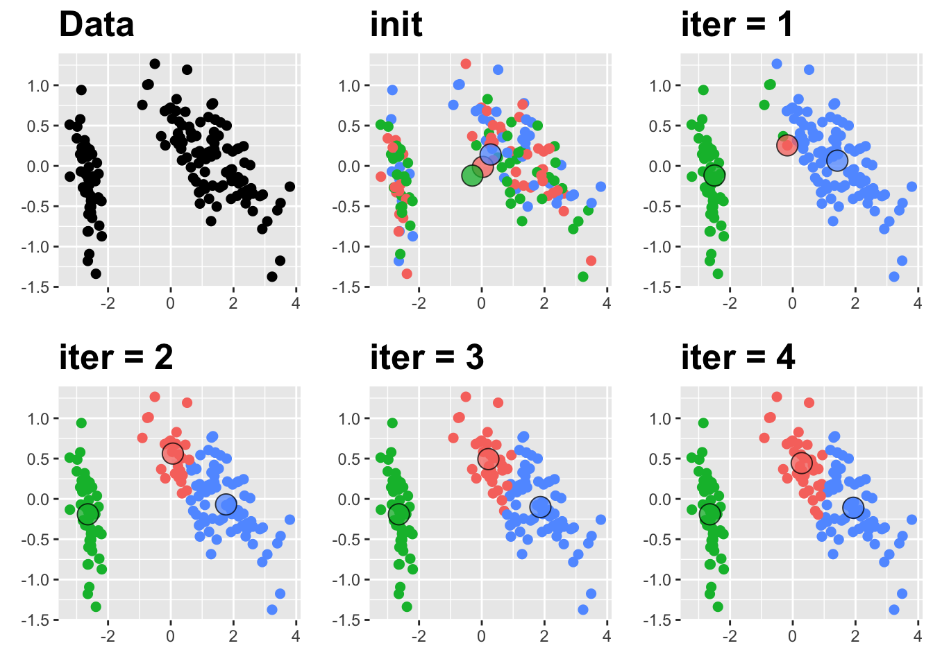
:::{.example name=“Lloyd’s algorithm and Iris Data} In this example, we’ll consider the three dimensional iris data. For visualization, we’ll plot the first two PC. Centers will be outlined in black.
 :::
:::
7.1.4 Strengths and Weaknesses
The advantages and disadvantages of center-based clustering algorithms can be separated into two main categories: computational and geometric. For now, we’ll focus on the computational aspects.
In the theoretical worst case, Lloyd’s algorithm can take\(\propto N^{k+1}\) iterations to converge, but it is typically very fast in practice. Most implementations, allow the user to set a maximum number of iterations and converge to approximate suboptimal solutions if the maximum number of iterations is reached. PAM and greedy \(k\)-center algorithms are typically much, much slower. However, once any of the clustering algorithms are complete, new data can be merged into cluster with nearest center. Other methods we’ll discuss later cannot incorporate new data without running the algorithm from scratch.
Ther are other issues that can increase the computational demands of center-based clustering. Each of the methods requires one to choose the number of clusters in advance. We discuss this issue in more depth shortly, but for now we want to emphasize that there is no connection between the \(k\)cluster solution and \((k+1)\) cluster solution. Thus, when investigating a suitable number of clusters, we need to run our clustering algorithm for a range of potential values of \(k\).
Convergence is also dependent on initial condition. In the figure below, we see two separate clustering arrangements resulting from different initial choices of the centers for \(k\)-means.

Thus, we also need to avoid convergence to local minima either by running many different initial conditions to convergence and picking the best solution or by using better initialization such as \(k\)-means++, which picks the initial points iteratively to maximize distance between the centers before running Lloyd’s algorithm. Using \(k\)-means++ can reduce the number of initializations that one should use, but does not eliminate the potential for convergence to a poor clustering. Thus, center-based algorithms can become quite computationally demanding analyze appropriately.
We have already discussed the impact of scale imbalance and outliers so as we turn to the geometric aspects of center based clustering, let’s first focus on the centers, which we often treat as representative examples of the cluster. However, the sample averages in \(k\)-means may not resemble actual data points. Though \(k\)-means may be much faster in prqctice, the centers in \(k\)-center and \(k\)-medoids are restricted to observations making them more representative of the data.
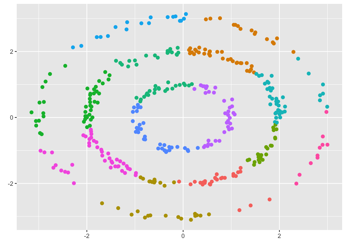
Clusters are based off interpretable notion of (Euclidean) distance so that points in a cluster are closer to one another than to points in other clusters. However, this feature biases center-based methods to clusters which are spherical in shape. If (dis)similarity not best captured through (squared) Euclidean distance, poor clustering is inevitable, and many of the methods used to estimate the number of cluster with tend to overestiamte the true value. As an example, consider the three rings shown at the beginning of this chapter. Silhouette scores (see 6.1.) suggest 12 clusters which is much larger than the three rings we see in the figure.
7.1.5 Choosing the number of clusters
There are many different methods which tend to give (slightly) different results. Direct methods such as the Elbow plot and silhouette diagnostics, are based on balancing a score measuring goodness of fit with a minimal number of clustering. Alternatively, one can consider testing methods such as the Gap Statistic which compare the clustering performance to a null model where clustering is absent.
7.1.5.1 Elbow plot
The center-based loss function will decrease as the number of clusters increases. Thus, we can plot the optimal loss found at different numbers of clusters and look for a sudden drop, much like we did with the scree plot in PCA. Below, we show an example of this method for data with three well separated spherical clusters
k <- 2:15
inertia <- rep(NA,length(k))
for (j in 1:length(k)){
  inertia[j] <- kmeans(data1,k[j])$tot.withinss
}
par(mfrow = c(1,2))
plot(data1$V1,data1$V2,xlab = '', ylab = '')
plot(k,inertia, ylab="k-means loss" )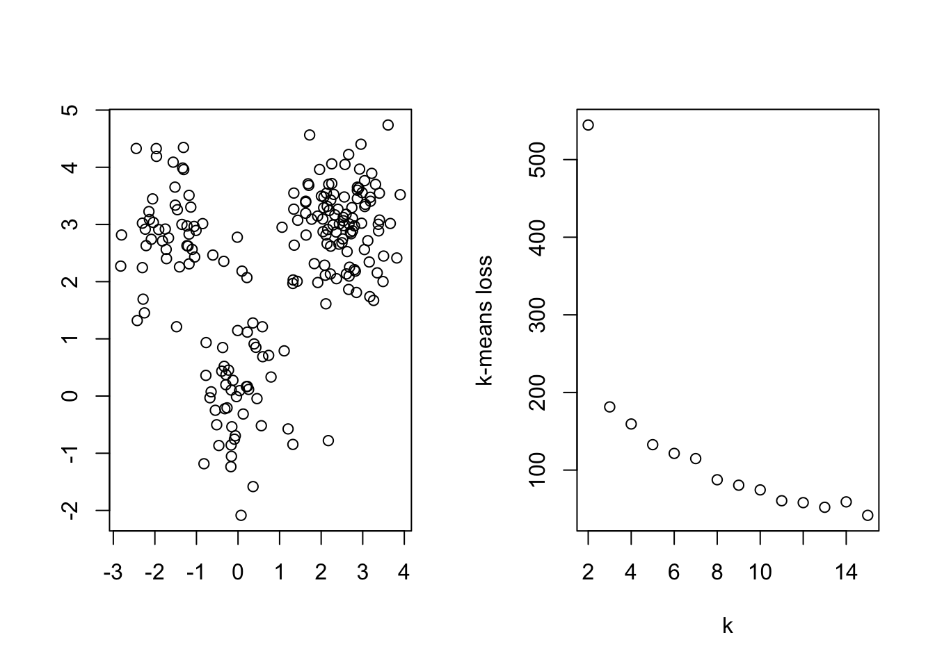
7.1.5.2 Gap Statistic
The Gap statistic (Tibshirani et al., (JRSS-B, 2001)), takes a specified number of clusters and compares the total within cluster variation to the expected within-cluster variation under the assumption that the data have no obvious clustering (i.e., randomly distributed). This method can be used to select an optimal number of clusters or as evidence that there is no clustering structure. Though best suited to center based methods (particularly \(k\)-means), one can apply it to the output of any clustering algorithm in practice so long as there is some quantitative measure of the quality of the clustering.
The algorithm proceeds through the following six steps.
Cluster the data at varying number of total clusters \(k\). Let \(L_{k-means}(k)\) be the total within-cluster sum of squared distances using \(k\) clusters.
Generate \(B\) reference data sets of size \(N\), with the simulated values of variable \(j\) uniformly generated over the range of the observed variable \(j\) . Typically \(B = 500.\)
For each generated data set \(b=1,\dots, B\) perform the clustering for each \(K\). Compute the total within-cluster sum of squared distances \(T_K^{(b)}\).
Compute the Gap statistic \[Gap(K) = \bar{w} - \log (T_K), \qquad \bar{w} = \frac{1}{B} \sum_{b=1}^B \log(T_K^{(b)})\]
Compute the sample variance \[var(K) = \frac{1}{B-1}\sum_{b=1}^B \left(\log(T_K^{(b)}) - \bar{w}\right)^2,\] and define \(s_K = \sqrt{var(K)(1+1/B)}\)
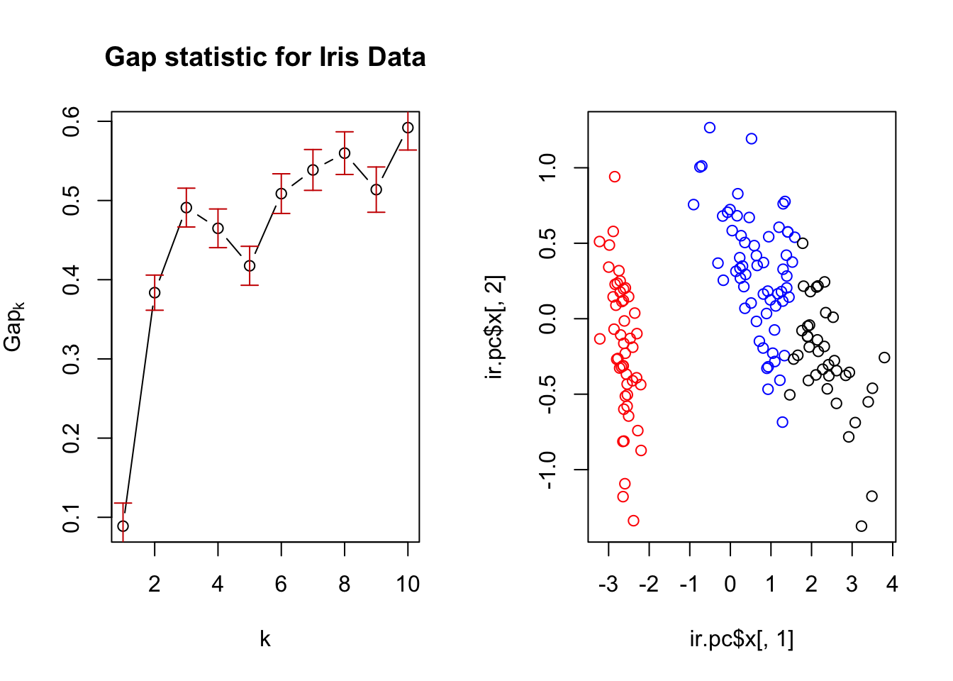
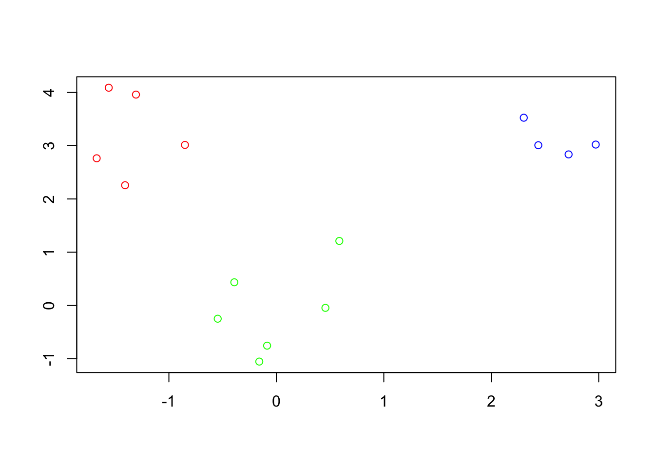
Finally, choose the number of clusters as the smallest K such that \[Gap(K) \ge Gap(K+1) - s_{K+1}\] ::: {.example name=“GAP statistic and iris data”} Below, we show a plot of the Gap Statistic (left) which indicates that three clusters is correct. The associated clustering is used to color a plot of the first two PC scores (right)
 :::
:::
7.1.5.3 Silhouette plots and coefficients
For a given clustering, we would like to determine how well each sample is clustered.
\[\begin{split} a_i &= \text{avg. dissimilarity of } \vec{x}_i \text{with all other samples in same cluster} \\ b_i &= \text{avg. dissimilarity of } \vec{x}_i \text{ with samples }\text{ in } the \text{ } closest \text{ cluster} \end{split}\]
We then define \[s_i = \frac{b_i - a_i}{\max\{a_i,b_i\}} \in (-1,1)\] as the silhouette for \(\vec{x}_i.\)
- Observations with \(s_i \approx 1\) are well clustered
- Observations with \(s_i \approx 0\) are between clusters
- Observations with \(s_i < 0\) are probably in wrong cluster
We can use any dissimilarity!
Can use silhouettes as diagnostics of any method!
A great clustering will have high silhouettes for all samples.
To compare different values of \(K\) (and different methods), we can compute the average silhouette \[S_K = \frac{1}{N}\sum_{i=1}^N s_i\] over a range of values of \(K\) and choose the \(K\) which maximizes \(S_K\).
7.2 Hierarchical Clustering
Hierarchical clustering views clustering from an alternative perspective compared to the partitioning viewpoint of center-based methods. Rather than finding an optimal paritioning of data into a pre-specified number of groups, hierarchical methods treat clustering as an iterative process either merging data into larger and larger groups (agglomerative methods) or dividing the full dataset into smaller and smaller clusters (divisive methods). As a result, there are strong connections between the clustering of data into \(k\) vs \(k+1\) groups. In particular, when using hierarchical methods, the optimal clustering of data into \(k\) (\(k+1\)) groups can be obtained by merging (splitting) the optimal clustering of data into \(k+1\) (\(k\)) groups.
7.2.1 Dendrograms
The key output of hierarchical clustering is a dendrogram (tree diagram) depicting the subsequent merges/divisions of data, where each merge/division is shown by a horizontal line, with height indicating dissimilarity between merged or divided clusters. Before discussing the generation of a dendrogram and the many choices on which the process depends, let’s first discuss how a dendrogram can be read and the information it provides for clustering.
In the figure below, samples 8 and 15 are merged into a cluster at height \(\approx 0.5\) indicating they have an original dissimilarity (Euclidean distance in this case) of 0.5. Sample 4 is then merged into the cluster with samples 8 and 15 at height \(\approx\) indicating the dissimilarity of sample 4 with the cluster of samples 8 and 15 is \(\approx 0.75\)
In addition to indicating the subsequent mergings/divisions of our data, the dendrogram can be used to determine a clustering of the data into a chosen number of clusters. For example, to cluster the data into three groups, we draw a horizontal line at a height (four in this case) which only cuts the tree into three branches.

Samples on the same branch are in the same cluster. Thus, the branch cut above suggest the following clustering:
- Cluster 1, samples: 12, 9, 13, 15, 2, 6
- Cluster 2, samples: 4, 5, 7, 8
- Cluster 3, samples: 3, 14, 10, 1, 11
which appears to match the clusters shown in the original data quite well.

7.2.2 Building a dendrogram
As suggested above there are two primary methods for building a dendrogram. The first is an aggolomerative approach which begins with \(N\) clusters (one per data point) then iteratively merges clusters based on the minimum dissimilarity until a final cluster containing all data remains. Alternatively, there is a divisive approach which begins with all data points in one cluster and splits iteratively until it finishes with \(N\) clusters (one per data point). Divisive clustering is less common, so we will focus on agglomerative methods hereafter.
Agglomerative clustering proceeds as follows.
- Initialize: Start with
Nclusters, one per data point. - Identify Closest Clusters: Find the pair with the smallest dissimilarity.
- Merge Clusters: Combine the clusters and recalculate distances.
- Repeat until only one cluster remains.
Importantly, the initial dissimilarity or distance is a tuneable choice made by the practitioners. While Euclidean distance is the default, the performance of the hierarchical agglomerative clustering is highly dependent on this choice. Like \(k\)-center and \(k\)-medoids clustering, you can non-Euclidean dissimilarities or distance such as Manhattan distance or cosine (dis)similarity if they would be a better choice depending on the application.
Additionally, we have also have a choice for specifying how the pairwise dissimilarities/distances are used to compute the distance between clusters containing more than one data point. The method for computing dissimilarity/distance between clusters is called linkage and common methods include
- Single Linkage: The distance between cluster \(A\) and cluster \(B\) is the smallest distance between a sample in \(A\) and a sample in \(B\). Using \(C_A\) and \(C_B\) to denote clusters \(A\) and \(B\), the distance between the clusters is \[d(C_A,C_B) = \min_{\vec{x}\in C_A, \vec{y} \in C_B} d(\vec{x},\vec{y}).\]
- Complete Linkage: The largest distance between a sample in \(A\) and a sample in \(B\) is used to define the distance between clusters \(A\) and \(B\). Mathematically, the distance between the clusters is \[d(C_A,C_B) = \max_{\vec{x}\in C_A, \vec{y} \in C_B} d(\vec{x},\vec{y}).\]
- Average Linkage: Average distance between all pairs of points in cluster \(A\) and \(B\) defines the cluster distance. Then, the distance between the clusters is \[d(C_A,C_B) = \frac{1}{|C_A|\,|C_B|}\sum_{\vec{x}\in C_A, \vec{y} \in C_B} d(\vec{x},\vec{y}).\]
- Ward’s Linkage: This method uses an iterative formula based on the squared distances to minimize the within cluster variation at each merge akin to \(k\)-means. When the input to agglomerative clustering is Euclidean distance, Ward’s Linkage is proportional to the squared Euclidean distance between the sample means in each cluster [37] though an explicit formula using the original dissimilarities is often used so that the original data is not required. For a complete discussion on this method and how it fits into the infinite family of Lance-Williams algorithms, see additional references [38, 39].
In the above, the notation \(d(\cdot,\cdot)\) represents the distance or dissimilarity of observations and/or clusters. Both the choice of original distances/dissimiliarities and the type of linkage have a strong impact on the quality of the clustering.
7.2.2.1 Comparing Linkage Methods
The four linkages methods above have different properties with single and complete representing extreme cases and average linkage and Ward linkage somewhere in between. Specifically, single linkage only requires two points to be close for clusters to merge, whereas complete linkage requires all pairs of points to be close. This “friend of my friend is my friend” feature of single linkage can generate clusters which are formed by long chains of singletons merged together at short heights and can in some cases capture manifold structure within a cluster. Conversely, complete linkage favors many small, compact clusters which get merged at larger heights.
Comparing and choosing a linkage method can use the above heuristics as a guide, but for a more data driven approach, Gap statistics or silhouette coefficients are suitable. Unique to hierarchical clustering, we can also use the cophenetic correlation as a quantitative measure of how well a clustering preserves pairwise distances/dissimilarities in the original data.
Definition 7.1 (Cophenetic Correlation Coefficient) For compactness, let \({\bf \Delta}_{ij}\), \(1\le i < j \le N,\) denote the user supplied distances/dissimilarities between observations \(i\) and \(j\). For a given choice of linkage, let \(h_{ij}\) be the height that \(\vec{x}_i\) and \(\vec{x}_j\) are merged into the same cluster. The cophenetic correlation is the sample correlation of the \(\binom{N}{2}\) pairs \[(h_{ij},{\bf \Delta}_{ij}), \qquad 1\le i < j \le N.\]
The cophenetic correlation can be computed for different linkage methods. Typically, the method closest to one (optimal value of the cophenetic correlation) should be selected, though care should be used as is the case with any method to balance additional factors.
7.2.2.2 Determining the number of clusters
In addition to selecting the number of clusters, Gap statistics and silhouette coefficients can also be used to select the optimal number of clusters. Other methods, such as the Mojena coefficient [40] are designed specifically for hierarchical clustering.
7.3 Model-Based Clustering
Unlike the preceding methods, model-based clustering assumes a probabilistic model for the data generating process. This model implies a likelihood (or posterior if we want to take a fully Bayesian approach) which we can optimize over the model parameters. Using the optimal parameters, we can construct probability weights for cluster membership (e.g. we assign sample one to cluster one with probability 0.6 and cluster two with probability 0.4) or make a discrete decision by assigning each sample to the cluster for which it has the highest probability of membership.
For now, fix the number of clusters as\(K\). Let us turn our attention to a standard two-step approach for generating a data set clustering structure which relies on two key components
- Cluster Densities: Each cluster is associated with a probability density \(f_j:\mathbb{R}^d \to \mapsto[0,\infty)\), for \(j=1,\dots,K\). (In the related literature, these densities are often referred to as kernels which should be confused with the kernels we have discussed previously.)
- Cluster Probabilities: Probabilities ${p_j}_{j=1}^K represent the a priori probability that a sample will be assigned to a given cluster
Now, suppose random vector \(\vec{x} \in \mathbb{R}^d\) is generated by first choosing a cluster label \(Z\) with probability \(p_j\), then conditional on \(Z=j\) we sample \(x\) from \(f_j\). This method implies the following joint density of \((\vec{x},z)\) \[\begin{equation} p(\vec{x},Z=j) = p_j f_j(\vec{x}) \end{equation}\] If we marginalize over \(z\), we then obtain the following mixture density for \(\vec{x}\), \[\begin{equation} p(\vec{x}) = \sum_{j=1}^K p_jf_j(\vec{x}) \end{equation}\]
We then repeat this approach independently \(N\) times to generate our data set. Hereafter, we’ll use \(Z_1,\dots,Z_n \in \{1,\dots,K\}\) to denote the latent cluster labels for each observation and continue using the notation \(\vec{x}_1,\dots,\vec{x}_N\) for our observed data. Under an independent sampling assumption, we then obtain the following joint distribution for the latent cluster labels and observed data \[\begin{equation} p(\vec{x}_1,Z_1=z_1,\dots,\vec{x}_N,z_N) = \prod_{i=1}^N p_{z_i} f_{z_i}(\vec{x}_i) \tag{7.1} \end{equation}\] When we turn to likelihood estimation, a slightly different expression of the likelihood will be helpful. We can rewrite (7.1) in the following form: \[\begin{align} p(\vec{x}_1,Z_1=z_1,\dots,\vec{x}_N,z_N) = \prod_{i=1}^N p_{z_i} f_j(\vec{x}_i) \\ &= \prod_{i=1}^N\sum_{j=1}^K \mathbb{1}(z_i=j)p_j f_j(\vec{x}_i) \\ &= \prod_{i=1}^N\prod_{j=1}^K \left[p_j f_j(\vec{x}_i)\right]^{\mathbb{1}(z_i=j)} \tag{7.2} \end{align}\] Marginalizing over \(Z_1,\dots,Z_N\) we then obtain the following joint density for the observed data \[\begin{equation} p(\vec{x}_1,\dots,\vec{x}_N) = \prod_{i=1}^N\left(\sum_{j=1}^K p_j f_j(\vec{x}_i)\right). \end{equation}\]
As in any modeling approach, performance is strongly influenced by the flexibility of the model to capture the observed data. There are many decisions which one can use to encode beliefs of the inherent structure of the data including the number of clusters, their shape, and the proportion of samples we expect in each cluster. For remainder of this section, we will focus on Gaussian mixture models (wherein \(f_1,\dots,f_K\) are Gaussian densities) which are the most common application of model-based clustering.
7.3.1 Gaussian Mixture Models (GMM)
For a fixed number of clusters \(k\), we assume that each cluster follows a Gaussian distribution, which are specified through their associated means and covariances. Following the notational convention from Chapter 2, we have \[f_j(\vec{x}) = \frac{1}{(2\pi)^{d/2}|{\bf \Sigma}_j|}\exp\left(-\frac{1}{2}(\vec{x}-\vec{\mu}_j)^T{\bf \Sigma}_j^{-1}(\vec{x}-\vec{\mu}_j)\right).\] Following the notational convention from chapter 2, we use the shorthand \[f_j(\vec{x}) = \mathcal{N}\left(\vec{x}; \,\vec{\mu}_j,{\bf \Sigma}_j\right).\] A Gaussian Mixture model (GMM) with \(K\) cluster is thus specified by the associated means, \(\{\vec{\mu}\}_{j=1}^K\), covariances matrices \(\{{\bf \Sigma}_j\}_{j=1}^K\) and probabilities \(p_1,\dots,p_K\). For brevity, we’ll use \[\Phi = \left\{ \{\vec{\mu}\}_{j=1}^K, \{{\bf \Sigma}_j\}_{j=1}^K, \{p_j\}_{j=1}^K \right\}\] to denote the set of model parameters. We’ll use \(p(\vec{x}_1,z_1,\dots,vec{x}_N,z_N \mid \Phi)\) to denote the joint distribution of the latent cluster labels and observations for a given set of parameters \(\Phi\). Similarly, we’ll use \(p(\vec{x}_1,\dots,\vec{x}_N \mid \Phi)\) to denote the marginal density of the observations given parameters \(\Phi\). Later, we’ll consider fixing \(\vec{x}_1,\dots,\vec{x}_N\) and treating \(p(\vec{x}_1,\dots,\vec{x}_N\mid\Phi)\) as a likelihood for \(\Phi\). First, let’s visualize data that can be generated by a GMM to demonstrate what shapes of clusters are possible for GMMs.
Example 7.2 (Samples from a GMM) Briefly, we’ll demonstrate the type of data one can generate from a Gaussian mixture model. We focus on a two-dimensional case with \(K=3\) clusters. For the sampling process, we’ll use means \[=\vec{\mu}_1 = \begin{bmatrix} 6 \\ 0 \end{bmatrix}, \, \vec{\mu}_2 = \begin{bmatrix} 0 \\ 3 \end{bmatrix}, \, \vec{\mu}_3 = \begin{bmatrix} -3 \\ 0 \end{bmatrix}\] and covariance matrices \[{\bf \Sigma}_1 = \begin{bmatrix} 1 & 0.5\\ 0.5 & 1 \end{bmatrix}, \, {\bf \Sigma}_2 = \begin{bmatrix} 0.5 & 0 \\ 0 &0.5 \end{bmatrix}, \, {\bf \Sigma}_3 = \begin{bmatrix} 5 & -3 \\ -3 & 2\end{bmatrix}\] for the Gaussian densities. And we’ll use probabilities \(\vec{p}=(0.5,0.3,0.2)\) for the cluster label assignment. Below, we show 1000 samples from this GMM with points color-coded by sampled cluster label \(z_i\).
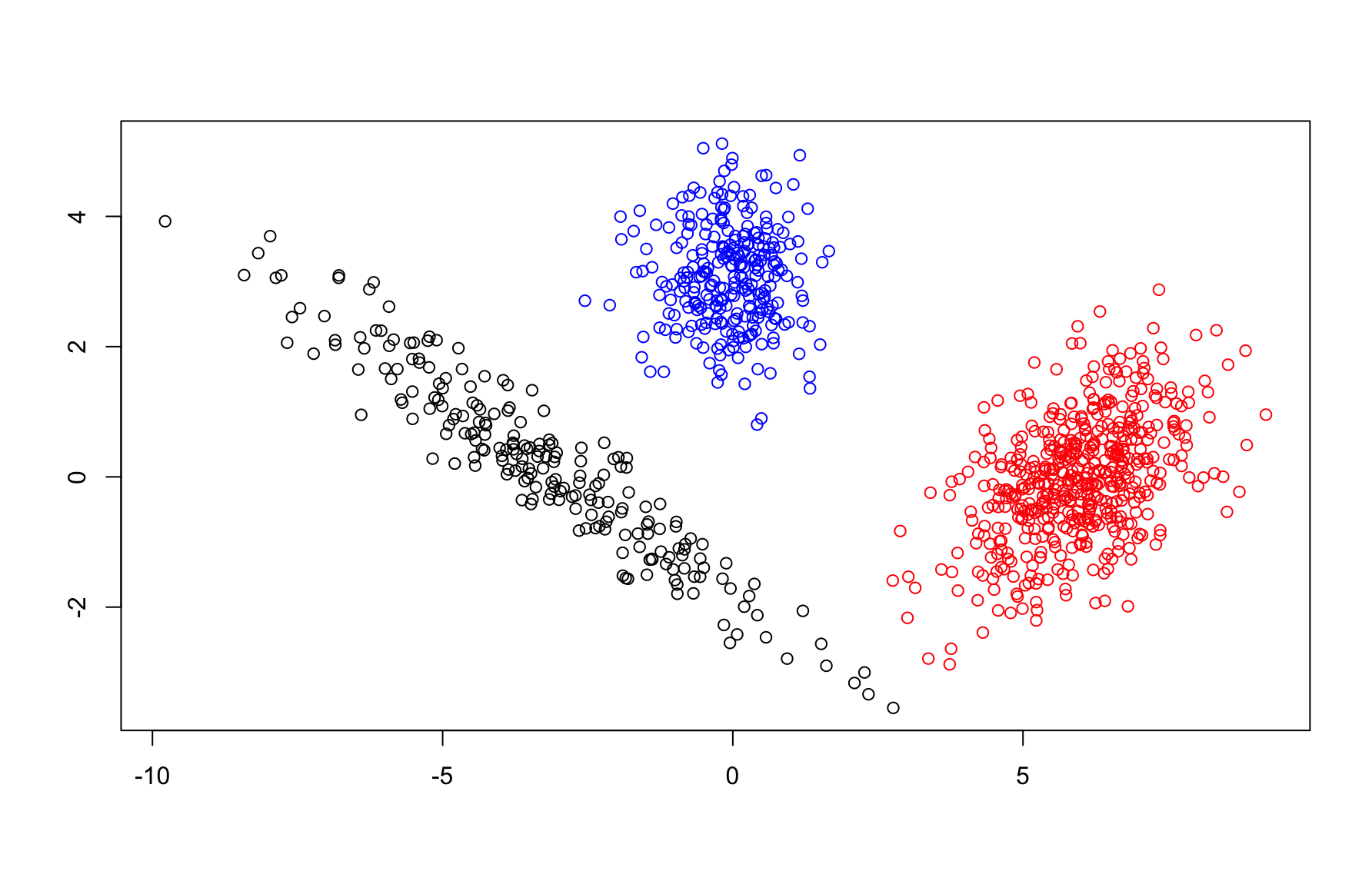
Figure 7.1: Samples from a GMM
In the preceding example, the clusters had an elliptical shape which is a distinct variation from \(k\)-means clustering which presumes spherical clusters. The location and shape/orientation of each cluster is controlled by its mean vector and covariance matrix respectively. As such, GMMs can still generate spherical clusters if the eigenvalues of each covariance matrix are (approximately) equal. This is a natural consequence of the Gaussian distribution and diagonalization of the covariance matrix. In high dimensions, Gaussian distributions concentrate near the surface of ellipsoids (rather than on the interior) but the general observation regarding the increased flexibility of GMMs over k-means holds true. Ignoring computational demands, one might expect GMMs to outperform k-means in many settings.
Suppose you were asked to assign a sample at the location marked with a purple x below.

Do you expect the x was generated from the same density as the points in the red cluster or from the density that generated the point in the black cluster? In center based clustering, this is a binary choice. However, it is unclear from the picture so perhaps that most honest answer is that there is a 50/50 chance that it was generated from either (we can likely agree there is vanishingly small chance it belongs to the blue cluster). The option to make such fuzzy clustering is a natural consequence of the probabilistic modeling approach behind GMMs. For a given parameter vector \(\Phi\) we can compute a posterior \(p(z_i | \vec{x}_i,\Phi)\) reflecting our belief about the clustering labeling.
Ultimately, clustering via GMMs requires estimation of the parameter \(\Phi\) for a given model. If we had access to the cluster labels, \(z_1,\dots,z_N\) this would be an easy problems. We could simply take sample means and covariances for the samples assigned to cluster \(j\) to estimate \(\vec{\mu}_j\) and \({\bf \Sigma}_j\) and we could use the proportion of samples given cluster label \(j\) as our estimate for \(p_j\). Mathematically, we would use the estimates \[\begin{equation} \hat{\mu}_j = \frac{\sum_{i=1}^N\mathbb{1}(Z_i=j)\vec{x}_i}{\sum_{i=1}^N\mathbb{1}(Z_i=j)}, \, \hat{\bf \Sigma}_j = \frac{\sum_{i=1}^N\mathbb{1}(Z_i=j)(\vec{x}_i-\hat{\mu_j})(\vec{x}_i-\hat{\mu_j})^T}{\sum_{i=1}^N\mathbb{1}(Z_i=j)}, \, \hat{p}_j = \frac{\sum_{i=1}^N\mathbb{1}(z_i=j)}{N} (\#eq:simple_gmm_estimates) \end{equation}\] where \(\mathbb{1}(z_i=j)\) is the indicator function taking value one if \(z_i=j\) and zero otherwise.
Unfortunately, we do not have access to \(z_1,\dots,z_N\). (If we did, there would be no need to estimate the clusters.) So we need an algorithm for optimizing \(p(\vec{x}_1,\dots,\vec{x}_N \mid \Phi)\) over \(\Phi\). One approach is to use a gradient based method to optimize the log-likelihood \[\begin{equation} \log p(\vec{x}_1,\dots,\vec{x}_N\mid \Phi) = \sum_{i=1}^N\log\left(\sum_{j=1}^N p_j\mathcal{N}(\vec{x}_i;\, \vec{\mu}_j,{\bf \Sigma}_j)\right). \end{equation}\] However, this method easily suffers from computation limitations (underflow) and additional care is required to enforce constraints on the parameters: the covariance matrices \(\{{\bf \Sigma}_j\}_{j=1}^K\) must be positive definite and the probabilities \(p_1,\dots,p_K\) must be non-negative and sum to one. Instead, we’ll use the powerful Expectation-Maximization (EM) algorithm which was named in the 1977 paper by Dempster, Laird, and Rubin [41]. In addition to proving convergence to a local maxima in our GMM setting, that paper also discusses many use cases for EM beyond mixture models.
7.3.2 Expectation-Maximization (EM) Algorithm
EM can be opaque when one is first exposed to the method. We’ll discuss the mathematical details shortly. For now, let’s discuss the algorithm from a high level. It begins with an initial guess for \(\Phi\). The EM algorithm is comprised of two aptly named steps.
- E-Step: We use our current guess for the model parameters to estimate the cluster labels \(z_1,\dots,z_N\). These estimates are probabilistic in the sense that we compute \(p(z_i\mid \vec{x}_i,\Phi)\) rather than discrete choices of the labels.
- M-Step: Maximize the expected log-likelihood with respect to parameters, \(\Phi\), using the estimated label probabilities. In this step, we modify the estimates in (eq:simple_gmm_estimates) to reflect our uncertainty in the cluster labels.
The EM algorithm then proceeds by iterating the E and M steps until convergence to a local maximum is achieved. Let’s explore these steps in greater detail for GMMs. Let \(\Phi^{(t)}\) to denote the estimate of \(\Phi\) after \(t\) iterations of the E and M steps. We’ll use the superscript \(^{(t)}\) above individual parameters as well.
In the E-step, we want to find \(p(z_i\mid \vec{x}_i, \Phi^{(t)})\) which follows from an application of Bayes’ formula \[\begin{align*} p(z_i=j\mid \vec{x}_i, \Phi^{(t)}) & = \frac{p(\vec{x}_i,z_i=j\mid \Phi^{(t)})}{p(\vec{x}_i\mid \Phi^{(t)})} \\ &= \frac{p(\vec{x}_i \mid z_i=j,\Phi^{(t)})p(z_i=j\mid \Phi^{(t)})}{p(\vec{x}_i\mid \Phi^{(t)})} \\ &= \frac{p_j^{(t)} \mathcal{N}(\vec{x}_i; \vec{\mu}^{(t)}_j,{\bf \Sigma}^{(t)}_j)}{\sum_{\ell=1}^Kp_\ell^{(t)} \mathcal{N}(\vec{x}_i; \vec{\mu}^{(t)}_\ell,{\bf \Sigma}^{(t)}_\ell)} \end{align*}\] We’ll adopt the notation \[\gamma_{ij}^{(t)} = \frac{p_j^{(t)} \mathcal{N}(\vec{x}_i; \vec{\mu}^{(t)}_j,{\bf \Sigma}^{(t)}_j)}{\sum_{\ell=1}^Kp_\ell^{(t)} \mathcal{N}(\vec{x}_i; \vec{\mu}^{(t)}_\ell,{\bf \Sigma}^{(t)}_\ell)}\] to compress our notation. Importantly, the quantities \(\gamma_{ij}^{(t)}\) give a conditional distribution of \(z_1,\dots,z_N\) given \(\vec{x}_1,\dots,\vec{x}_N\) and \(\Phi^{(t)}\)
Now, let’s turn to the handy form of the likelihood of the observations and the latent clusters labels in (7.2) which has associated log-likelihood \[\log p(\vec{x}_1,z_1,\dots,\vec{x}_N,z_N \mid \Phi) = \sum_{i=1}^N\sum_{j=1}^K \mathbb{1}(z_i =j) \log\left( p_j \mathcal{N}(\vec{x}_i; \vec{\mu}_j, {\bf \Sigma}_j)\right).\] Treating \(\vec{x}_1,\dots,\vec{x}_N\) and \(\Phi\) as fixed, we take the expectation of the above expression w.r.t. the cluster label probabilities \(\gamma_{ij}^{(t)}\). From the linearity of expectation, we have \[\begin{align*} Q(\Phi\mid \Phi^{(t)}) &= E_{z_1,\dots,z_N \mid \vec{x}_1,\dots,\vec{x}_N,\Phi^{(t)}}\left[ \log p(\vec{x}_1,z_1,\dots,\vec{x}_N,z_N \mid \Phi) \right] \\ &= \sum_{i=1}^N\sum_{j=1}^K \gamma_{ij}^{(t)} \log\left( p_j \mathcal{N}(\vec{x}_i; \vec{\mu}_j, {\bf \Sigma}_j)\right) \\ &= \sum_{i=1}^N\sum_{j=1}^K \gamma_{ij}^{(t)} \left[\log p_j -\frac{d}{2}\log(2\pi) - \frac{1}{2}\log |{\bf \Sigma}_j| - \frac{1}{2}(\vec{x}_i - \vec{\mu}_j)^T{\bf \Sigma}_j^{-1}(\vec{x}_i - \vec{\mu}_j) \right] \end{align*}\] The indicators \(\mathbb{1}(z_i=j)\) are replaced with the quantities \(\gamma_{ij}^{(t)}\) when we take the expectation! Once we have computed \(Q(\Phi\mid \Phi^{(t)})\) the E-step is complete.
For the \(M\)-step, we then optimize \(Q(\Phi\mid\Phi^{(t)})\) over \(\Phi\) so that \[\Phi^{(t+1)} = \text{argmax}_{\Phi}\,Q(\Phi\mid \Phi^{(t)}).\] For a GMM, there are closed form expressions for the optimal values of parameters. One can compute them directly using partial derivatives (and enforcing the constraints). We omit the calculation here and cite the result instead
\[\begin{align*} p_j^{(t+1)} &= \frac{\sum_{i=1}^N \gamma_{ij}^{(t)}}{\sum_{i=1}^N\sum_{\ell=1}^K \gamma_{i\ell}^{(t)}} = \frac{\sum_{i=1}^N\gamma_{ij}^{(t)}}{N} \\ \vec{\mu}_j^{(t+1)} &= \frac{\sum_{i=1}^N \gamma_{ij}^{(t)}\vec{x}_i}{\sum_{i=1}^N \gamma_{ij}^{(t)}} \\ {\bf \Sigma}_j^{(t+1)} &= \frac{\sum_{i=1}^N \gamma_{ij}^{(t)}(\vec{x}_i-\vec{\mu}_j^{(t+1)})(\vec{x}_i-\vec{\mu}_j^{(t+1)})^T}{\sum_{i=1}^N \gamma_{ij}^{(t)}} \end{align*}\]
The above quantities resemble the simple estimates from @ref(eq:simple_gmm_estimates). Rather than taking average using the known labels, we take weighted estimates using the relative probability of vectors have associated cluster labels!
Once we have computed \(\Phi^{(t+1)}\) when then return to the E-step and continuing iterating until convergence. Convergence of the EM algorithm to a local maximum follows directly from Jensen’s inequality [41]. Since the algorithm is only guaranteed to converge to a local maximum, one should typically investigate multiple initial conditions then select the parameter value among all optima that attains the highest log-likelihood \(p(\vec{x}_1,\dots,\vec{x}_N\mid \Phi)\).
Given a final estimate \(\Phi^*\) we can now determine a clustering of the data. Let \[\gamma_{ij}^* = \frac{p_j^{*} \mathcal{N}(\vec{x}_i; \vec{\mu}^*_j,{\bf \Sigma}^{*}_j)}{\sum_{\ell=1}^Kp_\ell^* \mathcal{N}(\vec{x}_i; \vec{\mu}^*_\ell,{\bf \Sigma}^*_\ell)}\] denote our estimate cluster label probabilities for each observation given parameter \(\Phi^*\). Each \(\gamma_{ij}^*\) reflects our belief that observation \(i\) was generated by the \(j\)th cluster density. To make a discrete clustering, we then assign observation \(\vec{x}_i\) to the cluster maximizing \(\gamma_{ij}^*\).
7.3.3 Model Selection and Parameter Constraints
The EM-algorithm provides a method for a finding the optimal parameters and subsequent clustering for a fixed number of clusters \(K\). If we wish to estimate the number of clusters, we can use the maximized log-likelihood as a measure of the goodness of fit to the data. Let \[\log L_k^* = \log p(\vec{x}_1,\dots,\vec{x}_N\mid \Phi^*)\] denote the maximum log-likelihood assuming \(k\) clusters. Larger values of \(\log L_k^*\) reflect a better fit to the observed data so it natural to expect \(\log L_k^*\) to increase as \(k\) increases. To avoid overfitting, we use the Bayesian Information Criterion (BIC). Let \(\mathcal{P}_k\) denote the number of parameters in a GMM for \(k\) clusters. BIC is defined as
\[BIC_k = 2 \log L_k^* - \mathcal{P}_k\log N \]
which balances goodness of fit with model complexity. Under this framework, we select the value of \(k\) which maximizes BIC. (Note, some sources define BIC as the negative of our formula above and select \(k\) opt to minimize. Be mindful of the convention when using pre-existing packages!)
We can use the BIC approach to investigate additional constraints on the model parameters. Recall from the 7.2, the shape of clusters is controlled by the covariance matrices. By applying addition constraints to \({\bf \Sigma}_1,\dots,{\bf \Sigma}_K\) we can reduce the number of model parameters. The standard convention for covariance constraints comes from Banfield and Raftery (1993) who observed that every covariance matrix can be decomposed via its eigenvalue decomposition \[{\bf \Sigma}_j = \lambda_j {\bf W}_j{\bf \Lambda}_j{\bf W}_j\] where \(\lambda_j\) is a scalar parameter controlling the volume of the cluster, \({\bf W}_j\) is an orthonormal matrix controlling the orientation of the cluster, and \({\bf \Lambda}_j\) is a diagonal matrix with diagonal entries in the interval \((0,1]\) giving the relative lengths of the semi-major axes of the ellipsoid [42]. We can apply constraints on one or more of the corresponding components of the covariance matrices summarized in the table below
| Volume | Shape | Orientation | |
|---|---|---|---|
| Equal | \[\lambda=\lambda_1=\dots=\lambda_K\] | \[\Lambda = \Lambda_1 = \dots = \Lambda_K\] | \[W=W_1=\dots W_K\] |
| Variable | \[\lambda_1,\dots,\lambda_K\] can differ | \[ \Lambda_1,\dots, \Lambda_K\] can differ | \[ W_1,\dots W_K\] can differ |
| Identity | Not applicable | \[\Lambda_1=\dots \Lambda_K = I\] | \[W_1=\dots W_K = I\] |
We then use triplets of qual, ariable, and dentity as shorthand for covariance constraints. For example, a GMM with covariance constraint EVE indicates covariances with equal volume, varying shape, and equal direction so that \[{\bf \Sigma}_j = \lambda {\bf W}{\bf \Lambda}_j{\bf W}^T.\] This results in a total of \(2\times 3\times 3 -4=14\) covariance options. We have subtracted 4 since some triplets coincide such as EII, EIE, and EIV.
For each covariance model, we can count the associated number of parameters and compute BIC accordingly. As a result, we have quantitative method for choosing the number of clusters and the optimal covariance model (for a given number of clusters). GMMs (with the help of the EM algorithm for fitting) provide a self-contained clustering framework with easy to interpret model selection criteria. However, there are inherent limitations which should be addressed.
7.3.4 Weakneses and Limitations
Unlike center-based methods, GMMs allow for a greater level of flexibility in the shapes of clusters (ellipses vs spheres). However, ellipsoids may still be inadequate choices a cluster supported on or near a nonlinear manifold. For example, in the smile data below.
Example 7.3 (GMMs fail to capture complex nonlinear structure) Consider the following data in \(\mathbb{R}^2\) which exhibitis four clusters upon visual inspection
The eyes and nose are each compact and approximately elliptical in shape, but the mouth is concentrated around a nonlinear parabolic curve. Applying the GMM model above for a range \(K=2,\dots,15\) clusters gives the following BIC curves
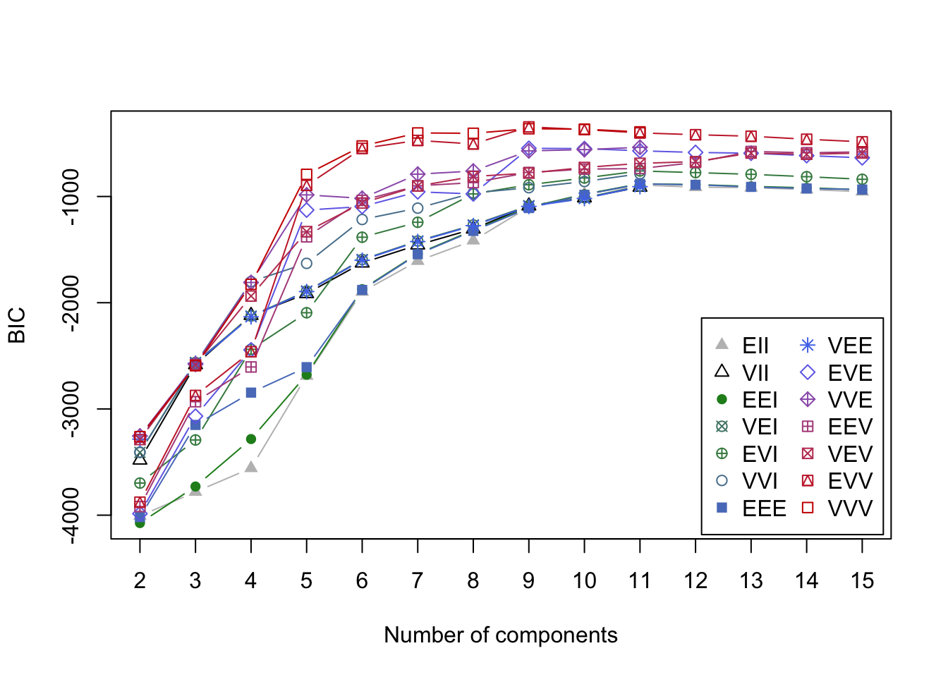
Figure 7.2: BIC curves for GMMs applied to the smile data
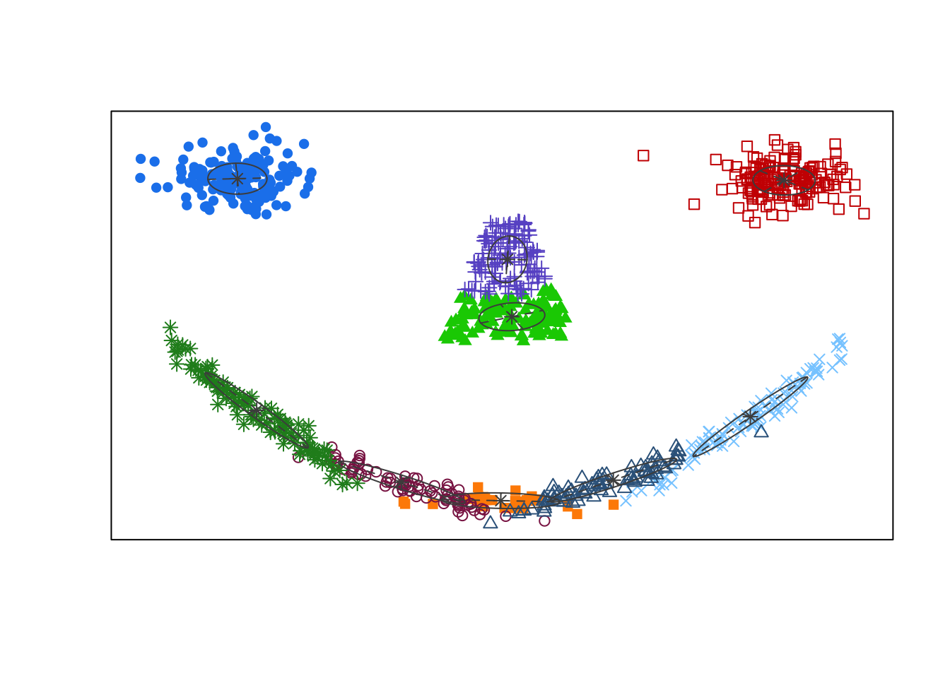
Using BIC, the optimal GMM one should select contains nine clusters with EVV covariance structure. In the associated clustering shown below, the eyes are appropriately clustered, but the nose is split into two separate clusters. Most egregiously though, we can see the mouth was broken apart into five thin elliptic pieces reflecting the inherent limitations of the cluster shapes that can be identified by GMMs.
Given this limitation, there has been considerable work dedicated to improving model-based clustering including the design of more expressive mixture densities [[43];[44];[45]} and methods which produce more parsimonious clustering arrangements by iteratively merging nearby clusters [46].
7.4 Spectral Clustering
7.4.1 Introduction
Spectral Clustering represents a significant leap in the evolution of clustering techniques. Distinguished from traditional methods like K-means, it excels in detecting complex structures and patterns within data. It’s based on ideas from graph theory and simple math concepts, mainly focusing on how to use information from graphs. Imagine each piece of data as a point on a graph, with lines connecting the points that are similar. Spectral Clustering uses these connections to figure out how the data should be grouped, which is especially handy when the groups are twisted or oddly shaped.
The key step in Spectral Clustering is breaking down a special graph matrix (called the Laplacian matrix) to find its eigen values and eigen vectors. These eigen vectors help us see the data in a new way that makes the groups more obvious. This makes it easier to use simple grouping methods like K-means to sort the data into clusters. This approach is great for finding hidden patterns in the data.
However, Spectral Clustering comes with its own challenges. Choosing the right number of groups can be tricky, and it might not work as well with very large sets of data because of the relatively large computing cost. Nevertheless, its robustness and adaptability have cemented its role across various domains, from image processing to bioinformatics.
7.4.2 Algorithm
Similarity Graph Construction: Start by constructing a similarity graph \(G\) from your data (similar to the steps in Laplacian Eigenmap section. Each data point is represented as a node in the graph.)
Define the edges of the graph. There are three common ways to do this:
\(\epsilon\)-neighborhood graph: Connect all points whose pairwise distances are smaller than \(\epsilon\).
K-nearest neighbors: For each point, connect it to its k nearest neighbors.
Fully connected graph: Connect all points with each other. Typically, the Gaussian similarity function (also known as the Radial Basis Function or RBF) is used to calculate the weights of the edges: \(w_{ij} = \exp(-\frac{||\vec{x}_i - \vec{x}_j||^2}{2\sigma^2})\), where \(\vec{x}_i\) and \(\vec{x}_j\) are two points in the dataset and \(\sigma\) is a tuning parameter.
Note:It is worth noting that there exists a slight difference in the construction of similarity graph matrix compared to Laplacian Eigenmap we mentioned in manifold learning chapter. For the fully connected graph, after using Radial basis to depict all the pair-wise distances, we don’t need to set a threshold and sparsify the matrix (set some entries to zero) like we did in Laplacian Eigenmap, we just keep all the original radial basis distances.
Graph Laplacian Matrix: Similar to corresponding parts in Laplacian Eigenmap. Calculate the adjacency matrix \(W\), where \(W_{ij}\) represents the weight of the edge between nodes \(i\) and \(j\). Calculate the degree matrix \(D\), which is a diagonal matrix where each diagonal element \(D_{ii}\) is the sum of the weights of the edges connected to node \(i\). Compute the unnormalized Graph Laplacian matrix \(L\) as \(L = D - W\).
Eigen Decomposition: Perform the eigen decomposition on the Laplacian matrix \(L\) to find its eigenvalues and eigenvectors. Select \(k\) smallest eigenvalues and their corresponding eigen vectors. \(k\) is the number of clusters you want to identify.
Mathematical Proof behind this step
As we have stated in Laplacian Eigenmap section, the Graph Laplacian matrix \(L\) is positive semi-definite.
Given any vector \(\vec{y} \in \mathbb{R}^N\)
\[ \vec{y}^T \mathbf{L} \vec{y}=\frac{1}{2}\sum_{i=1}^N \sum_{j=1}^N \mathbf{W}_{i j}\left(y_i-y_j\right)^2 \]
Obviously, it is non-negative. Besides, we can always find a vector \(\vec{y} = \mathbf{1}_N\) that makes it zero, which means the smallest eigen value must be zero, with the corresponding eigen vector being \(\mathbf{1}\).
From the above equation, we can also justify our eigen-decomposition approach in finding the number of clusters. For either \(\epsilon\)-neighborhood graph or K-nearest neighbors approach, if point \(i\) and \(j\) are not connected, then \(\mathbf{W}_{ij}=0\), however, if they are connected, \(\mathbf{W}_{ij} = 1 > 0\). With some careful observation, we find that as long as we set \(y_i=y_j\) for \(\forall \mathbf{W}_{ij} > 0\), then we are able to get zero in the above equation. Since in cluster \(\Omega_1 = \{\vec{x}_p, \dots , \vec{x}_q \}\), all the points are connected, and \(\mathbf{W}_{ij} > 0 \; \forall \{\vec{x}_i, \vec{x}_j\} \in \Omega_1\), we can simply set \(y_i=1\) for \(\; \forall i \in \Omega_1\), and \(y_j=0\) for \(\; \forall j \notin \Omega_1\). So the eigen-vector that corresponds to cluster \(\Omega_1\) is \(\vec{y}_1 = \sum \vec{e}_i \in \mathbb{R}^N, \; \forall \, i \; s.t. \vec{x}_i \in \Omega_1\), where \(\vec{e}_i\) is a vector with all zero except the \(i^{th}\) entry being one.
So when we perform eigen decomposition on Graph Laplacian matrix \(\mathbf{L}\): \(\mathbf{L} = \mathbf{Q} \mathbf{\Lambda} \mathbf{Q}^T\). Then for \(\vec{y}\) s.t. \(\vec{y}^T \mathbf{L} \vec{y}=0\), we can rewrite it as
\[ \vec{y}^T \mathbf{L} \vec{y} = \vec{y}^T \mathbf{Q} \mathbf{\Lambda} \mathbf{Q}^T \vec{y} = (\mathbf{\Lambda}^{1/2} \mathbf{Q}^T \vec{y})^T (\mathbf{\Lambda}^{1/2} \mathbf{Q}^T \vec{y})=0 \] As a result, we know \(\mathbf{\Lambda}^{1/2} \mathbf{Q} \vec{y} = \vec{0}\), in other words
\[ \mathbf{L} \vec{y} = \mathbf{Q} \mathbf{\Lambda} \mathbf{Q}^T \vec{y} = (\mathbf{Q} \mathbf{\Lambda}^{1/2})(\mathbf{\Lambda}^{1/2} \mathbf{Q}^T \vec{y}) = \vec{0} \] So we know that \(\vec{y}\) is just an eigen-vector of \(\mathbf{L}\), with the corresponding eigen-value being zero.
In reality, especially when we use Fully-connected graph, we can’t get \(k\) exact zero-eigenvalues with corresponding \(k\) eigenvectors. (Different clusters are not necessarily completely separate, and Fully-connected graph even allows every \(\mathbf{W}_{ij} > 0\)). So we will just conduct eigen decomposition and choose \(k\) smallest eigenvalues together with their corresponding eigen-vectors.
A toy example
First, we’ll create the simulation data with two distinct clusters.
Visualize the data points to make it more intuitive.
plot(data, col = c(rep("red", nrow(cluster1)), rep("blue", nrow(cluster2))), pch = 19, xlab = "X-axis", ylab = "Y-axis")
text(data, labels = 1:nrow(data), pos = 4, col = "black")  # Adding labels
title("Data Points Visualization")
We use the \(\epsilon\)-neighborhood approach to construct the similarity graph.
##      [,1] [,2] [,3] [,4] [,5] [,6]
## [1,]    0    1    1    0    0    0
## [2,]    1    0    1    0    0    0
## [3,]    1    1    0    0    0    0
## [4,]    0    0    0    0    1    1
## [5,]    0    0    0    1    0    1
## [6,]    0    0    0    1    1    0
Compute the Laplacian matrix.
degree_matrix <- diag(apply(similarity_matrix, 1, sum))
laplacian_matrix <- degree_matrix - similarity_matrix
print(laplacian_matrix)
## [,1] [,2] [,3] [,4] [,5] [,6]
## [1,] 2 -1 -1 0 0 0
## [2,] -1 2 -1 0 0 0
## [3,] -1 -1 2 0 0 0
## [4,] 0 0 0 2 -1 -1
## [5,] 0 0 0 -1 2 -1
## [6,] 0 0 0 -1 -1 2Perform eigen decomposition on the Laplacian matrix. We choose the smallest two eigenvalues here since we want to
eigen_result <- eigen(laplacian_matrix)

# Sort eigenvalues and their corresponding eigenvectors
sorted_indices <- order(eigen_result$values)
sorted_eigenvalues <- eigen_result$values[sorted_indices]
sorted_eigenvectors <- eigen_result$vectors[, sorted_indices]

# Select the smallest two eigenvalues and their corresponding eigenvectors
smallest_eigenvalues <- sorted_eigenvalues[1:2]
smallest_eigenvectors <- sorted_eigenvectors[, 1:2]
print(smallest_eigenvalues)
## [1] 1.776357e-15 1.776357e-15## [,1] [,2]
## [1,] 0.0000000 -0.5773503
## [2,] 0.0000000 -0.5773503
## [3,] 0.0000000 -0.5773503
## [4,] -0.5773503 0.0000000
## [5,] -0.5773503 0.0000000
## [6,] -0.5773503 0.0000000We find that the smallest two eigen-values are 0 (not exact zero here because of computational precision issue), and their corresponding eigen-vectors give us information about the clustering. The first cluster contains data point 4, 5, 6; while the second cluster contains the rest three data points 1, 2, 3.
We try fully-connected graph with radial basis function to construct the adjacency matrix this time.
gamma <- 1  # Scale parameter for the RBF kernel
n <- nrow(data)
similarity_matrix <- matrix(0, n, n)

for (i in 1:n) {
  for (j in 1:n) {
    if (i != j) {
      distance <- dist(rbind(data[i, ], data[j, ]))^2
      similarity_matrix[i, j] <- exp(-gamma * distance)
    }
  }
}

print(similarity_matrix)
## [,1] [,2] [,3] [,4] [,5] [,6]
## [1,] 0.000000e+00 2.865048e-01 6.065307e-01 1.522998e-08 2.172440e-10 2.289735e-11
## [2,] 2.865048e-01 0.000000e+00 2.865048e-01 8.764248e-08 1.522998e-08 2.172440e-10
## [3,] 6.065307e-01 2.865048e-01 0.000000e+00 3.726653e-06 8.764248e-08 1.522998e-08
## [4,] 1.522998e-08 8.764248e-08 3.726653e-06 0.000000e+00 2.865048e-01 6.065307e-01
## [5,] 2.172440e-10 1.522998e-08 8.764248e-08 2.865048e-01 0.000000e+00 2.865048e-01
## [6,] 2.289735e-11 2.172440e-10 1.522998e-08 6.065307e-01 2.865048e-01 0.000000e+00degree_matrix <- diag(apply(similarity_matrix, 1, sum))
laplacian_matrix <- degree_matrix - similarity_matrix
print(laplacian_matrix)## [,1] [,2] [,3] [,4] [,5] [,6]
## [1,] 8.930355e-01 -2.865048e-01 -6.065307e-01 -1.522998e-08 -2.172440e-10 -2.289735e-11
## [2,] -2.865048e-01 5.730097e-01 -2.865048e-01 -8.764248e-08 -1.522998e-08 -2.172440e-10
## [3,] -6.065307e-01 -2.865048e-01 8.930393e-01 -3.726653e-06 -8.764248e-08 -1.522998e-08
## [4,] -1.522998e-08 -8.764248e-08 -3.726653e-06 8.930393e-01 -2.865048e-01 -6.065307e-01
## [5,] -2.172440e-10 -1.522998e-08 -8.764248e-08 -2.865048e-01 5.730097e-01 -2.865048e-01
## [6,] -2.289735e-11 -2.172440e-10 -1.522998e-08 -6.065307e-01 -2.865048e-01 8.930355e-01eigen_result <- eigen(laplacian_matrix)
# Sort eigenvalues and their corresponding eigenvectors
sorted_indices <- order(eigen_result$values)
sorted_eigenvalues <- eigen_result$values[sorted_indices]
sorted_eigenvectors <- eigen_result$vectors[, sorted_indices]
# Select the smallest two eigenvalues and their corresponding eigenvectors
smallest_eigenvalues <- sorted_eigenvalues[1:2]
smallest_eigenvectors <- sorted_eigenvectors[, 1:2]
print(smallest_eigenvalues)## [1] 2.564067e-16 2.632047e-06## [,1] [,2]
## [1,] -0.4082483 0.4082488
## [2,] -0.4082483 0.4082494
## [3,] -0.4082483 0.4082467
## [4,] -0.4082483 -0.4082467
## [5,] -0.4082483 -0.4082494
## [6,] -0.4082483 -0.4082488As we can see, this time the two smallest eigenvalues are not both zero, with one being a little bit more than zero. This has something to do with the properties of the new adjacency matrix \(\mathbf{A}\). In addition, we observe that the the two eigen-vectors are not something we expected. It seems weird at the first glance, but since \(\mathbf{L} \vec{y} = \vec{0}\), \(\vec{y} = \vec{y}_2 \pm \vec{y}_1\) is also an eigen-vector with the eigen-value being zero, we are still able to recover the two clusters. This suggests us that we may do some computation ourselves after getting the eigen-vectors to recover the clustering situation.
In this situation, it may seem that fully-connected graph is not as straight-forward as the other two adjacency matrix construction methods, and the result is also not as optimal. But we should realize that in real-data situation, different clusters are not totally separate, as a result, a soft-threshold can be a better choice in most situations.