Chapter 4 Linear Methods
4.1 Principal Component Analysis
Principal component analysis (PCA) is arguably the first method for dimension reduction, which dates back to papers by some of the earliest contributors to statistical theory including Karl Pearson and Harold Hotelling [6, 7]. Pearson’s original development of PCA borrowed ideas from mechanics which provides a clear geometric/physical interpretation of the resulting PCA loadings, variances, and scores, which we will define later. This interpretability and an implementation that uses scalable linear algebra methods – allowing PCA to be conducted on massive datasets – is one of the reasons PCA is still used prolifically to this day. In fact, many more modern and complex methods still rely on PCA as an internal step in their algorithmic structure.
There are number of different but equivalent derivations of PCA including the minimization of least squares error, covariance decompositions, and low rank approximations. We’ll revisit these ideas later, but first, let’s discuss PCA through a geometrically motivated lens via a method called iterative projections.
4.1.1 Derivation using Iterative Projections
We begin with a data matrix \[{\bf X} = \begin{bmatrix} \vec{x}_1^T\\ \vdots \\\vec{x}_N^T\end{bmatrix} \in\mathbb{R}^{N\times d}.\] Let’s begin with an example of dimension reduction where we’ll seek to replace each vector \(\vec{x}_1,\dots,\vec{x}_N\) with corresponding scalars \(y_1,\dots,y_N\) which preserve as much of the variability between these vectors as possible. To formalize this idea, let’s introduce a few assumptions.
First, we’ll assume the data \(\vec{x}_1,\dots,\vec{x}_N\) are centered. To be fair, assumption may be too strong a word. Rather, it’s a first step in preprocessing that will simplify the analysis later. We’ll discuss how to account for this centering step later, but for now assume \(\bar{x} = \vec{0}\) so that \({\bf HX} = {\bf X}\). More importantly, let’s assume that each \(y_i\) is constructed in the same way. Specifically, let \(y_i = \vec{x}_i^T \vec{w}\) for some common vector \(\vec{w}\). Thus, we can view each one-dimensional representation as a dot product of the corresponding observed vector with the same vector \(\vec{w}.\) We can compactly write this expression as \[\vec{y} = \begin{bmatrix}y_1\\ \vdots \\ y_n \end{bmatrix}=\begin{bmatrix}\vec{x}_1^T \vec{w} \\ \vdots \\ \vec{x}_N^T \vec{w}\end{bmatrix} = {\bf X} \vec{w}.\]
How do we choose \(\vec{w}\)? We would like differences in the scalars \(y_1,\dots,y_N\) to reflect differences in the vectors \(\vec{x}_1,\dots,\vec{x}_N\) so having \(y_1,\dots,y_N\) spread out is a natural goal. Thus, if \(\vec{x}_i\) and \(\vec{x}_j\) are far apart then so will \(y_i\) and \(y_j\). To do this, we’ll try to maximize the sample variance of the \(y\)’s. The sample variance \[\frac{1}{N} \sum_{i=1}^N (y_i - \bar{y})^2 = \frac{1}{N}\sum_{i=1}^N(\vec{x}_i^T \vec{w} - \bar{y})^2\] will depend on our choice of \(\vec{w}\). In the previous expression, \[\bar{y} = \frac{1}{N} y_i = \frac{1}{N}\sum_{i=1}^N \vec{x}_i^T \vec{w} = \frac{1}{N}\vec{1}^T{\bf X}\vec{w}\] is the sample mean of \(y_1,\dots,y_N.\) Importantly, since we have assumed that \(\vec{x}_1,\dots,\vec{x}_N\) are centered, it follows that \(\bar{y}=0\) and the sample variance of \(y_1,\dots,y_N\) simplifies to \[\frac{1}{N}\sum_{i=1}^N(\vec{x}_i^T \vec{w})^2 = \frac{1}{N}\sum_{i=1}^N y_i^2 = \frac{1}{N} \|y\|^2 = \frac{1}{N}\vec{y}^T\vec{y}.\]
We can write the above in terms of \({\bf X}\) and \(\vec{w}\). Using the identity \(\vec{y} = {\bf X}\vec{w}\), we want to choose \(\vec{w}\) to maximize \[\frac{1}{N}\vec{y}^T\vec{y} = \frac{1}{N}({\bf X}\vec{w})^T{\bf X}\vec{w} = \frac{1}{N}\vec{w}^T{\bf X}^T{\bf X}\vec{w} = \vec{w}^T\left(\frac{{\bf X}^T{\bf X}}{N}\right)\vec{w}.\] Since we have assumed that \({\bf X}\) is centered it follows that \({\bf X}^T{\bf X}/N\) is the sample covariance matrix \(\hat{\bf \Sigma}\)! Thus, we want to make \(\vec{w}^T\hat{\bf \Sigma} \vec{w}\) as large as possible.
Naturally, we could increase the entries in \(\vec{w}\) and increase the above expression without bound. To make the maximization problem well posed, we will restrict \(\vec{w}\) to be unit-length under the Euclidean norm so that \(\|\vec{w}\|=1.\) We now have a constrained optimization problem which gives rise to the first principal component loading.
Definition 4.1 (First PCA Loading and Scores) The first principal component loading is the vector \(\vec{w}_1\) solving the constrained optimization problem \[\begin{equation} \begin{split} \text{Maximize } &\vec{w}^T \hat{\bf \Sigma}\vec{w} \\ \text{subject to constraint } &\|\vec{w}\|=1. \end{split} \end{equation}\] The first principal component scores are the projections, \(y_i = \vec{x}_i^T\vec{w}_1\) for \(i=1,\dots, N\), of each sample onto the first loading.
To find the first PCA loading we can make use of Lagrange multipliers (see exercises) to show that \(\vec{w}_1\) must also satisfy the equation \[\hat{\bf \Sigma}\vec{w}_1 = \lambda \vec{w}_1\] where \(\lambda\) is the Lagrange multiplier. From this expression, we can conclude that the first principal component loading is the unit length eigenvector associated with the largest eigenvalue of the sample covariance matrix \(\hat{\bf \Sigma}\) and that the Lagrange multiplier \(\lambda\) is the largest eigenvalue of \(\hat{\bf \Sigma}\). In this case, we refer to \(\lambda\) as the first principal component variance.
4.1.1.1 Geometric Interpretation of \(\vec{w}_1\)
Since \(\|\vec{w}_1\| = 1\) we may interpret this vector as specifying a direction in \(\mathbb{R}^d\). Additionally, we can decompose each of our samples into two pieces: one pointing in the direction specified by \(\vec{w}_1\) and a second portion perpendicular to this direction. Thus, we may write \[\vec{x}_i = \underbrace{\vec{w}_1 \vec{x}_i^T\vec{w}_1}_{parallel} + \underbrace{(\vec{x}_i -\vec{w}_1 \vec{x}_i^T\vec{w}_1)}_{perpendicular}.\] By the Pythagorean theorem, \[\begin{align*} \|\vec{x}_i\|^2 &= \| \vec{w}_1 \vec{x}_i^T\vec{w}_1 \|^2 + \|\vec{x}_i -\vec{w}_1 \vec{x}_i^T\vec{w}_1\|^2 \\ &= (\vec{w}_1^T\vec{x}_i)^2 + \|\vec{x}_i -\vec{w}_1 \vec{x}_i^T\vec{w}_1\|^2 \\ &= y_i^2 + \|\vec{x}_i -\vec{w}_1 \vec{x}_i^T\vec{w}_1\|^2 \end{align*}\] for \(i=1,\dots,N\). Averaging over all of samples gives the expression \[\frac{1}{N}\sum_{i=1}^N\|\vec{x}_i\|^2 = \frac{1}{N}\sum_{i=1}^N y_i^2 +\frac{1}{N}\sum_{i=1}^N \|\vec{x}_i -\vec{w}_1 \vec{x}_i^T\vec{w}_1\|^2.\] The left-hand side of the above expression is fixed for a given set of data, whereas the first term on the right side is exactly what we sought to maximize when finding the first principal component loading. This quantity is the average squared length of the projection of each sample onto the direction \(\vec{w}_1\). As such, we can view the first principal component loading as the direction in which \(\vec{x}_1,\dots,\vec{x}_N\) most greatly varies. Let’s turn to an example in \(\mathbb{R}^3\) to view this.
Example 4.1 (Computing the First PCA Loading and Scores) Below, we show a scatterplot of \(N=500\) points in \(\mathbb{R}^3\) drawn randomly from a MVN. These data have been centered.
Notice the oblong shape of the cloud of points. Rotating this image, it is clear that the data varies more in certain directions than in others.
The sample covariance matrix of these data is \[ \hat{\Sigma} = \begin{bmatrix} 11.4&7.12&3.22 \\ 7.12&9.21&9.03 \\ 3.22&9.03&15.99 \\ \end{bmatrix} \] We can use the eigendecomposition of this matrix to find the first PCA loading and variance. Given the first loading we can also compute the first PCA scores. A short snippet of code for this calculation is shown below.
Sigmahat <- (t(data) %*% data)/N # calculate the sample covariance matrix, recall the data has been centered
Sigmahat.eigen <- eigen(Sigmahat) # calculate the eigen decomposition of Sigmahat
y <- data %*% Sigmahat.eigen$vectors[,1] # calculate the scores
The largest eigenvalue (first PC variance) is \(\lambda = 25.58\) with associated eigenvector \((-0.44, -0.57, -0.69)^T\) which is the first PC loading.
We can visualize these results in a few different ways. First, we can add the span of \(\vec{w}_1\) (shown in red) to the scatterplot of the data. One can see that \(\vec{w}_1\) is oriented along the direction where the data is most spread out.Figure 4.1: Samples with Span of First Loading
We could also generate a scatterplot of the scores, but we’ll show these scores along the \(\vec{w}_1\) axes so that they correspond to the projection of each sample onto span\(\{\vec{w}_1\}\); equivalently, we are plotting the vectors \(y_i \vec{w}_i\).
Figure 4.2: Decomposition of Samples into Components Parallel and Perpendicular to First Loading
4.1.1.2 Additional Principal Components
The first PCA loading provides information about the direction in which are data most greatly vary, but it is quite possible that there are still other directions wherein our data still exhibits a lot of variability. In fact, the notion of a first principal component loading, scores, and variance suggests the existence of a second, third, etc. iteration of these quantities. To explore these quantities, let’s proceed as follows
For each datum, we can remove its component in the direction of \(\vec{w}_1\), and focus on the projection onto the orthogonal complement of \(\vec{w}_1\). Let \[\vec{x}_i^{(1)} = \vec{x}_i - \vec{w}_1\vec{x}_i^T\vec{w}_1 = \vec{x}_i - \vec{w}_1 y_i\] denote the portion of \(\vec{x}_i\) which is orthogonal to \(\vec{w}_1\). These points are shown on the right side of Fig @{fig:pca1}. Here, the superscript \(^{(1)}\) indicates we have removed the portion of each vector in the direction of the first loading.
We can organize the orthogonal components into a new data matrix \[{\bf X}^{(1)} = \begin{bmatrix} \left(\vec{x}_1^{(1)}\right)^T \\ \vdots \\ \left(\vec{x}_N^{(1)}\right)^T \end{bmatrix} = \begin{bmatrix} \vec{x}_1^T - \vec{x}_1^T\vec{w}_1\vec{w}_1^T \\ \vdots \\ \vec{x}_N^T - \vec{x}_N^T\vec{w}_1\vec{w}_1^T \end{bmatrix} = {\bf X} - {\bf X}\vec{w}_1\vec{w}_1^T.\] Now let’s apply PCA to the updated data matrix \({\bf X}^{(1)}\) from which we get the second principal component loading, denoted \(\vec{w}_2\), the second principal component scores, and the second principal component variance. One can show that the data matrix \({\bf X}^{(1)}\) is centered so that its sample covariance matrix is \[\begin{equation} \hat{\bf \Sigma}^{(1)} = \frac{1}{N}({\bf X}^{(1)})^T{\bf X}^{(1)}. \end{equation}\] The 2nd PC variance is the largest eigenvalue of \(\hat{\bf \Sigma}^{(1)}\) and its associated unit length eigenvector is the 2nd PC loading, denoted \(\vec{w}_2\). The second PC scores \(\vec{w}_2^T\vec{x}_i^{(1)}\) for \(i=1,\dots,N.\)
Continuing ??, we have \[ \hat{\bf \Sigma}^{(1)} = \begin{bmatrix} 6.36&0.61&-4.61 \\ 0.61&0.81&-1.07 \\ -4.61&-1.07&3.86 \\ \end{bmatrix} \] which has largest eigenvalue 10.02 (2nd PC variance) and associated eigenvector \(\vec{w}_2 = (0.78, 0.12, -0.61)^T\) (2nd PC Loading). The second set of PC scores are given by \(\vec{w}_2^T\vec{x}_i^{(1)}\) for \(i=1,\dots, N.\)
Here is one crucial observation. The vector \(\vec{w}_2\) gives the direction of greatest variability of the vectors \(\vec{x}_1^{(1)},\dots,\vec{x}_N^{(1)}.\) For each of these vectors we have removed the component in the direction of \(\vec{w}_1\). Thus, \(\vec{x}_1^{(1)},\dots,\vec{x}_N^{(1)}\) do not vary at all in the \(\vec{w}_1\) direction. What can we say about \(\vec{w}_2\)? Naturally, it must be perpendicular to \(\vec{w}_1\)! We can see this geometric relationship if we plot the vectors \(\vec{x}^{(1)}_i\) in our previous example along with the span of the first and second loading.
Figure 4.3: First and 2nd Loadings with Data after component along first loading has been removed
We need not stop at the second PCA loading, scores, and variance. We could remove components in the direction of \(\vec{w}_2\) and apply PCA to the vectors \[\begin{align*} \vec{x}_i^{(2)} &= \vec{x}_i^{(1)} - \vec{w}_2 (\vec{x}_i^{(1)})^T\vec{w}_2\\ &= \vec{x}_i - \vec{w}_1\vec{x}_i^T\vec{w}_1 - \vec{w}_2(\vec{x}_i - \vec{w}_1\vec{x}_i^T\vec{w}_1)^T\vec{w}_2\\ &= \vec{x}_i - \vec{w}_1\vec{x}_i^T\vec{w}_1 - \vec{w}_2\vec{x}_i^T\vec{w}_2 + \vec{w}_2\vec{w_1}^T\vec{x}_i\underbrace{\vec{w}_1^T\vec{w}_2}_{=0} \end{align*}\] which gives rise to the centered data matrix \[\begin{equation} {\bf X}^{(2)} = \begin{bmatrix} \vec{x}_1^T- \vec{w}_1^T\vec{x}_1\vec{w}_1^T - \vec{w}_2^T\vec{x}_1\vec{w}_2^T \\ \vdots \\ \vec{x}_d^T- \vec{w}_1^T\vec{x}_d\vec{w}_1^T - \vec{w}_2^T\vec{x}_d\vec{w}_2^T \end{bmatrix} = {\bf X} - {\bf X}\vec{w}_1\vec{w}_1^T - {\bf X}\vec{w}_2\vec{w}_2^T \end{equation}\] with corresponding covariance matrix \[\hat{\Sigma}^{(2)} = \frac{1}{N}({\bf X}^{(2)})^T{\bf X}^{(2)}\] from which we can obtain a third loading (\(\vec{w}_3\)), variance (\(\lambda_3)\), and set of scores \(\vec{w}_3\vec{x}_i^{(2)}\) for \(i=1,\dots,N\).
We can continue repeating this argument \(d\) times for our \(d\)-dimensional data until we arrive at a set of \(d\) unit vectors \(\vec{w}_1,\dots,\vec{w}_d\) which are the \(d\) PCA loadings. Why do we stop after \(d\)? The principal component loadings \(\vec{w}_1,\dots,\vec{w}_d\) are all mutually orthogonal and unit length so they form an orthonormal basis for \(\mathbb{R}^d\). All of the variability in each sample can be expressed in terms of these \(d\) basis vectors.
This iterative approach is admittedly, to intensive for most practical applications. Fortunately, we do not need to follow the sequence of projections and then eigenvalue computations thanks to the following theorem.
Theorem 4.1 Suppose \(\vec{w}_1,\dots,\vec{w}_d\) are the orthonormal eigenvectors of the sample covariance \(\hat{\Sigma}=\frac{1}{N}{\bf X}^T{\bf X}\) with eigenvalues \(\lambda_1\ge \dots\ge \lambda_d \ge 0\) respectively, i.e. \(\hat{\Sigma}\vec{w}_j = \lambda_j\vec{w}_j\). Then \(\vec{w}_1,\dots,\vec{w}_d\) are also eigenvectors or the matrix \(\hat{\Sigma}^{(1)}=\frac{1}{N}({\bf X}^{(1)})^T{\bf X}^{(1)}\) with eigenvalues \(0,\lambda_2,\dots,\lambda_d\) respectively.
This result follows nicely from the geometric observation that the loadings are mutually orthogonal. The second loading is then the eigenvector associated with the second largest eigenvalue of the original covariance matrix. Taking the orthogonality of the loadings further, we can get even more from the following corollary.
Corollary 4.1 Suppose \(\vec{w}_1,\dots,\vec{w}_d\) are the orthonormal eigenvectors of the sample covariance \(\hat{\Sigma}=\frac{1}{N}{\bf X}^T{\bf X}\) with eigenvalues \(\lambda_1\ge \dots\ge \lambda_d \ge 0\) respectively. Then for \(k=2,\dots,d-1\), the vectors\(\vec{w}_1,\dots,\vec{w}_d\) are also eigenvectors of the matrix \(\hat{\Sigma}^{(k)}=\frac{1}{N}({\bf X}^{(k)})^T{\bf X}^{(k)}\) with eigenvalues \(\underbrace{0,\dots,0}_k,\lambda_{k+1},\dots,\lambda_d\) respectively.
As a result, we can immediately compute the PCA variances and loadings given the full spectral (eigenvalue) decomposition \[\begin{equation} \hat{\Sigma} = \begin{bmatrix} \vec{w}_1 & | & \dots & | &\vec{w}_d \end{bmatrix} \begin{bmatrix} \lambda_1 &0 & 0 \\ 0 &\ddots & 0 \\ 0 & 0 &\lambda_d \end{bmatrix} \begin{bmatrix} \vec{w}_1^T \\ \vdots \\\vec{w}_d^T \end{bmatrix}. \end{equation}\]
Again, thanks to orthogonality, we can also compute the PCA scores directly from the original data without iteratively removing components of each vector in the direction of the various loadings. To summarize PCA, given data \({\bf X}\) we first compute the spectral decomposition of the sample covariance matrix \(\hat{\bf \Sigma}\). The eigenvalues (in decreasing magnitude) provide the PC variance and the corresponding unit-length eigenvectors give the corresponding loadings, which form an orthonormal basis in \(\mathbb{R}^d\). The PC scores are the inner product of each vector with these loadings (assuming the data are centered). Thus, the PCA scores are \(\vec{x}_i^T\vec{w}_1,\dots,\vec{x}_i^T\vec{w}_d\) for \(i=1,\dots,d.\) We can compactly (again assuming our data are centered) express the scores in terms of the original data matrix and the loadings as
\[\begin{equation} {\bf Y} = {\bf XW} \end{equation}\]
where \({\bf Y}\in \mathbb{R}^{N\times d}\) is a matrix of PC scores and \({\bf W}\) is the orthonormal matrix with columns given by the loadings.
4.1.1.3 Geometric interpretation of PCA
We began with an \(N\times d\) data matrix \({\bf X}\) and now we have an \(N\times d\) matrix of PCA scores \({\bf Y}\). One may be inclined to ask: where is the dimension reduction? To answer this question, let’s revisit some important features of the scores and loadings.
First, since the loadings \(\vec{w}_1,\dots,\vec{w}_d\) are orthonormal vectors in \(\mathbb{R}^d\), they naturally form a basis! The PCA scores are then the coordinates of our data in the basis \(\{\vec{w}_1,\dots,\vec{w}_d\}\). Specifically, \({\bf Y}_{ij}\) for \(j=1,\dots,d\) are the coordinates for (centered) vector \(\vec{x}_i\) since \[\vec{x}_i = {\bf Y}_{i1}\vec{w}_1+\cdots+ {\bf Y}_{id}\vec{w}_d.\]
The dimension reduction comes in from an important observations about the PCA scores (aka coordinate). Consider the sample covariance matrix of the PCA scores, which one can show is diagonal (see exercises)
\[\begin{equation} \hat{\bf \Sigma}_Y = \begin{bmatrix} \lambda_1 & & \\ &\ddots & \\ && \lambda_d \end{bmatrix} \end{equation}\]
There are two important perspectives on the using PCA scores. First, the diagonality of the PCA scores indicates that in the new basis, \(\{\vec{w}_1,\dots,\vec{w}_d\}\), the coordinates are i) uncorrelated and ii) ordered in decreasing variance. As a result, if we want to construct a \(k < d\) dimensional representation our data that minimizes the loss in variability, we should use the first \(k\) PCA scores.
Secondly, we can use the first \(k\) scores to build approximations, \[\vec{x}_i \approx \hat{x}_i = {\bf Y}_{i1}\vec{w}_1+\cdots + {\bf Y}_{ik} \vec{w}_k, \qquad i=1,\dots, N.\] How good is this approximation? Optimal, in a squared loss sense, thanks to the following theorem.
Theorem 4.2 Fix \(k<d.\) Given any \(k\)-dimensional linear subspace of \(\mathbb{R}^d\), denoted \(\mathcal{V}\), let \(\text{proj}_{\mathcal{V}}(\vec{x})\) denote the orthogonal projection of \(\vec{x}\) onto \(\mathcal{V}\), then \[\frac{1}{N}\sum_{i=1}^N \|\vec{x}_i - \text{proj}_{\mathcal{V}}(\vec{x}_i)\|^2 \ge \lambda_{k+1}+\cdots+\lambda_d\] where \(\lambda_{k+1},\cdots,\lambda_d\) are the last \((d-k)\) principal component variances of \(\vec{x}_1,\dots,\vec{x}_N\).
Furthermore, if \(\lambda_k > \lambda_{k+1}\), then \(\text{span}\{\vec{w}_1,\dots,\vec{w}_k\}\) is the unique \(k\)-dimensional linear subspace for which \[\frac{1}{N}\sum_{i=1}^N \|\vec{x}_i - \text{proj}_{\mathcal{V}}(\vec{x}_i)\|^2 = \lambda_{k+1}+\cdots+\lambda_d.\]
A few notes on the above theorem to add some clarity. First, note that \[\hat{x}_i = {\bf Y}_{i1}\vec{w}_1+\cdots + {\bf Y}_{ik} \vec{w}_k\] is the orthogonal projection of \(\vec{x}_i\) onto \(\text{span}\{\vec{w}_1,\dots,\vec{w}_k\}\) so that \[\vec{x}_i - \text{proj}_{\text{span}\{\vec{w}_1,\dots,\vec{w}_k\}}(\vec{x}_i) = {\bf Y}_{i,k+1}\vec{w}_{k+1}+\cdots+{\bf Y}_{id}\vec{w}_d.\] Using this identity and the properties of the PCA scores allows one to verify the equality at the end of the theorem (see exercises).
The requirement that \(\lambda_k\ge \lambda_{k+1}\) is necessary for uniqueness. If \(\lambda_k = \lambda_{k+1}\) then the subspace \(\text{span}\{\vec{w}_1,\dots,\vec{w}_{k-1},\vec{w}_{k+1}\}\) would offer an equally good approximation. Fortunately, it is rare that two (nonzero) PCA scores are equal in practice so we rarely have to worry about this issue. In short, PCA learns the \(k\)-dimensional linear subspace which best approximates the original data on average!
In all of the previous analysis, we have been operating under the assumption that our data is centered, e.g. \(\bar{x}=\vec{0}\) – an preprocessign step that made our analysis easier and is done in practice to avoid potential issue with numerical linear albegra. We can recover all of the nice geometric intuition when working with uncentered data by adding the sample mean back to the approximation and shifting our focus to affine subspaces, which look just like linear subspaces which have been translated by some constant shift away from the origin.
::: {.corollary $pca-opt-aff} Given any \(k\)-dimensional affine subspace \(\mathcal{A}\subset\mathbb{R}^d\) \[\frac{1}{N}\sum_{i=1}^N \|\vec{x}_i - \text{proj}_{\mathcal{A}}(\vec{x}_i)\|^2 \ge \lambda_{k+1}+\cdots+\lambda_d\] with equality (assuming \(\lambda_k>\lambda_{k+1}\)) if and only if \(\mathcal{A} = \bar{x} + \text{span}\{\vec{w}_1,\dots,\vec{w}_k\}.\) :::
Note the set \(\bar{x} + \text{span}\{\vec{w}_1,\dots,\vec{w}_k\}\) is the set of all vectors \[\{\vec{v}\in\mathbb{R}^d:\,\vec{v}-\bar{x} \in \text{span}\{\vec{w}_1,\dots,\vec{w}_k\}\},\] i.e. the optimal \(k\)-dimensional hyperplane found after centering if translated by \(\hat{x}\). In this case, the optimal approximation of our data is \[\vec{x}_i \approx \bar{x} + {\bf Y}_{i1}\vec{w}_1+\cdots + {\bf Y}_{ik}\vec{w}_k.\]
4.1.2 PCA in Practice
4.1.2.1 Choosing the number of components
Now that we have explored the mathematical details of PCA, let us turn to practical guidance when working with real data.
A natural first question for PCA, is how many principal components should I use? Like many modeling decisions in statistics there are a range of answers from simple heuristics to advanced technical answers. For PCA, methods based on random matrix theory are quite strong but also beyond the scope of this book. The curious reader is encouraged to see [8] for more information. Herein, we are going to focus on simpler but more common approaches with an emphasis on inherent trade-offs. Like many statistical modeling choices, decisions are not always so clear cut, and it’s best to understand and reason about decisions in the context of a specific problem rather than following hard and fast rules.
The best known method for choosing an optimal number of principal components is the scree plot [9], which is based on a visual inspection of a plot of the principal component variances in decreasing order. Ideally, one would observe an elbow delineating a regions where the variances decrease sharply then saturate near a small value.
library("ggrepel")
df <- data.frame(lambda = c(15,10,5,2,1.25,1,1,1,1,1,1,1,1,1,1), comp = 1:15)
elbow_point <- 5
ggplot(df, aes(x=comp, y = lambda)) + geom_point() + xlab("Component, k") +
  ylab(expression(lambda[k])) +
  ggtitle("Scree plot") +
  theme_minimal() +
  # Annotate the elbow point
  geom_text_repel(aes(label = ifelse(comp == elbow_point, "elbow", "")),
                  nudge_y = 5,
                  arrow = arrow(length = unit(0.015, "npc")))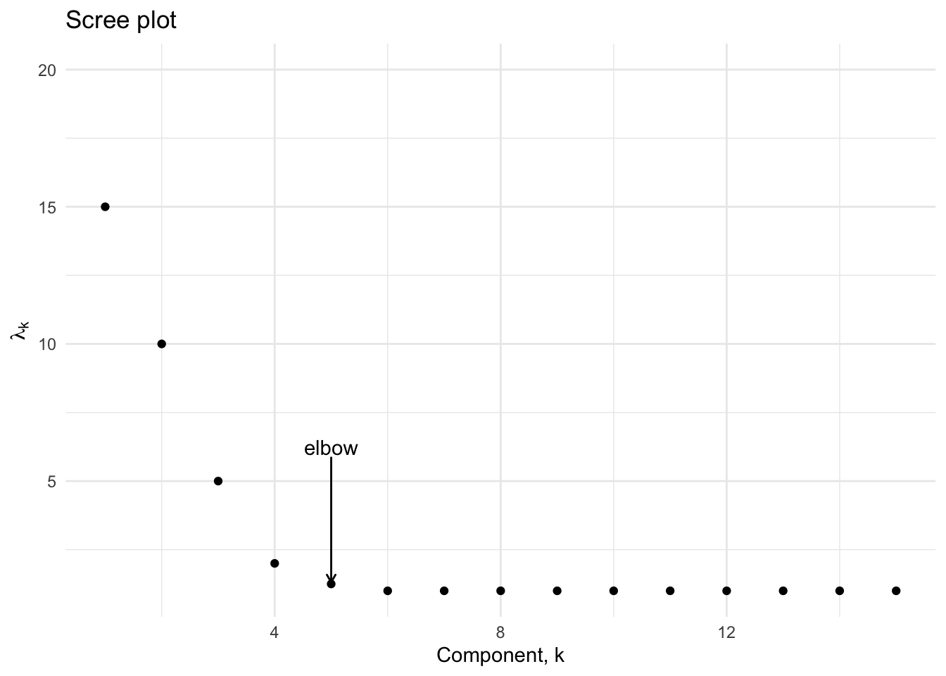
Figure 4.4: Idealized version of the scree plot
In the preceding figure, we would opt to keep the first four components since the variance appears to saturate beginning with the fifth principal component.
Another heuristic suggests keeping the number of components needed to explain a specified percentage of the variance, typically 80 or 90%. Using 80% as a guide would suggest keeping the first 7 principal components (using the first 6 only gets us to 79.2%) based on the related figure below.
Using the same data as above, we have the following percentage explained variance plot below
df$varp = cumsum(df$lambda)/sum(df$lambda)
ggplot(df, aes(x=comp, y = varp)) + geom_point() + xlab("Component, k") +
ylab("% of explained variance") 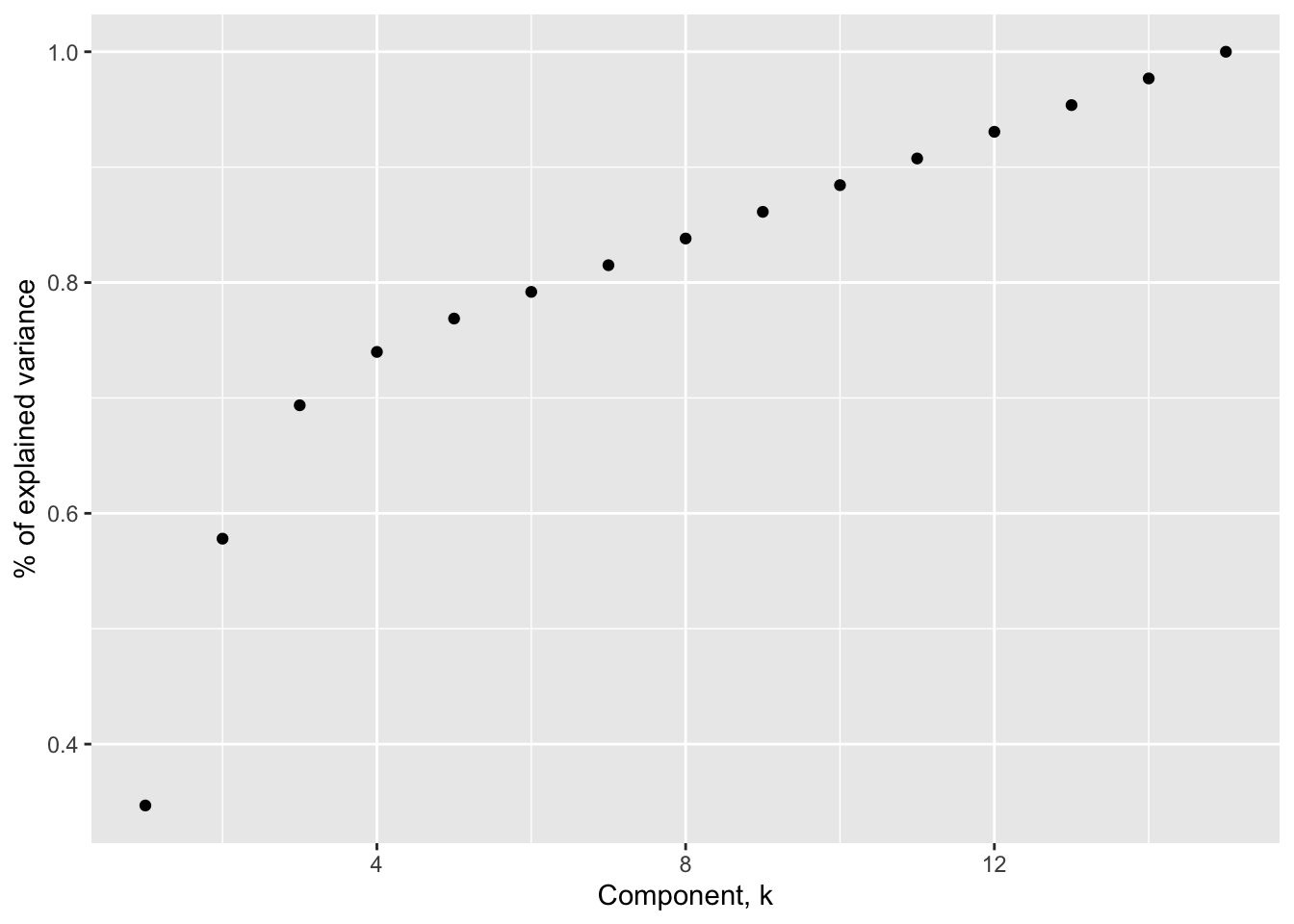
Figure 4.5: Percentage of explained variance
Specifically, we have plotted the cumulative sum of the p.c. variances relative to the total variance \[\frac{\sum_{j=1}^k \lambda_j}{\sum_{j=1}^d \lambda_j} = \frac{\sum_{j=1}^k \lambda_j}{tr(\hat{\bf \Sigma}_x)}\] as a function of the number of components.
Based on an evaluation of the principal component variances we have two heuristics suggesting different cutoffs (4 vs. 7). Which (if either) is correct? Like many issues in statistics, the answer depends on context. Perhaps there is a data driven reason to choose 4 or 7 or some other number for that matter. The important issue is to recognize the inherent trade-off in the choice so that one can make the best decision in the context of the larger data science problem where PCA is being applied. Choosing a smaller (larger) number of components gives a greater level of dimension reduction at the expense of worse (better) approximation and retention of variability.
Additionally, the variances alone often are not enough to understand the structure of your data. As we will see in the next section, in some cases you may observe as stark drop in variances that is the result of features of data unrelated to concentration near a lower dimensional hyperplane.
4.1.2.2 Limitations and vulnerabilities
PCA relies on sample variance of data projected in different direction. As such, it is susceptible to outliers and/or imbalanced scales which can greatly influence calculations of sample variance. Furthermore, PCA is optimal at finding the best linear subspace as shown in the preceding sections. However, it cannot find (potentially simpler and more compressed) nonlinear structure in the data. Let’s investigate each of these limitations in the following subsections.
4.1.2.2.1 Imbalanced scales
As a motivating example, let’s consider the wine dataset which contains observations of 13 chemical compounds (variables) for 178 different wines (subjects) from three different cultivars. Below we show the first 10 rows of the data matrix.
| Alcohol | MalicAcid | Ash | AlcAsh | Mg | Phenols | Flav | NonFlavPhenols | Proa | Color | Hue | OD | Proline |
|---|---|---|---|---|---|---|---|---|---|---|---|---|
| 14.23 | 1.71 | 2.43 | 15.6 | 127 | 2.80 | 3.06 | 0.28 | 2.29 | 5.64 | 1.04 | 3.92 | 1065 |
| 13.20 | 1.78 | 2.14 | 11.2 | 100 | 2.65 | 2.76 | 0.26 | 1.28 | 4.38 | 1.05 | 3.40 | 1050 |
| 13.16 | 2.36 | 2.67 | 18.6 | 101 | 2.80 | 3.24 | 0.30 | 2.81 | 5.68 | 1.03 | 3.17 | 1185 |
| 14.37 | 1.95 | 2.50 | 16.8 | 113 | 3.85 | 3.49 | 0.24 | 2.18 | 7.80 | 0.86 | 3.45 | 1480 |
| 13.24 | 2.59 | 2.87 | 21.0 | 118 | 2.80 | 2.69 | 0.39 | 1.82 | 4.32 | 1.04 | 2.93 | 735 |
| 14.20 | 1.76 | 2.45 | 15.2 | 112 | 3.27 | 3.39 | 0.34 | 1.97 | 6.75 | 1.05 | 2.85 | 1450 |
| 14.39 | 1.87 | 2.45 | 14.6 | 96 | 2.50 | 2.52 | 0.30 | 1.98 | 5.25 | 1.02 | 3.58 | 1290 |
| 14.06 | 2.15 | 2.61 | 17.6 | 121 | 2.60 | 2.51 | 0.31 | 1.25 | 5.05 | 1.06 | 3.58 | 1295 |
| 14.83 | 1.64 | 2.17 | 14.0 | 97 | 2.80 | 2.98 | 0.29 | 1.98 | 5.20 | 1.08 | 2.85 | 1045 |
| 13.86 | 1.35 | 2.27 | 16.0 | 98 | 2.98 | 3.15 | 0.22 | 1.85 | 7.22 | 1.01 | 3.55 | 1045 |
Prior to running PCA, we might be able to guess which coordinates account for the most variability. Proline (on the scale of 1000s) and magnesium (on the scale of 100s) have much larger values than other coordinates in the data matrix. We can see this observation holds out immediately when looking at the biplot summarizing PCA run on the wine data.
library(ggbiplot)
out <- prcomp(wine)
ggbiplot(out, scale = 0, varname.color = "red")  +ylim(c(-250,250))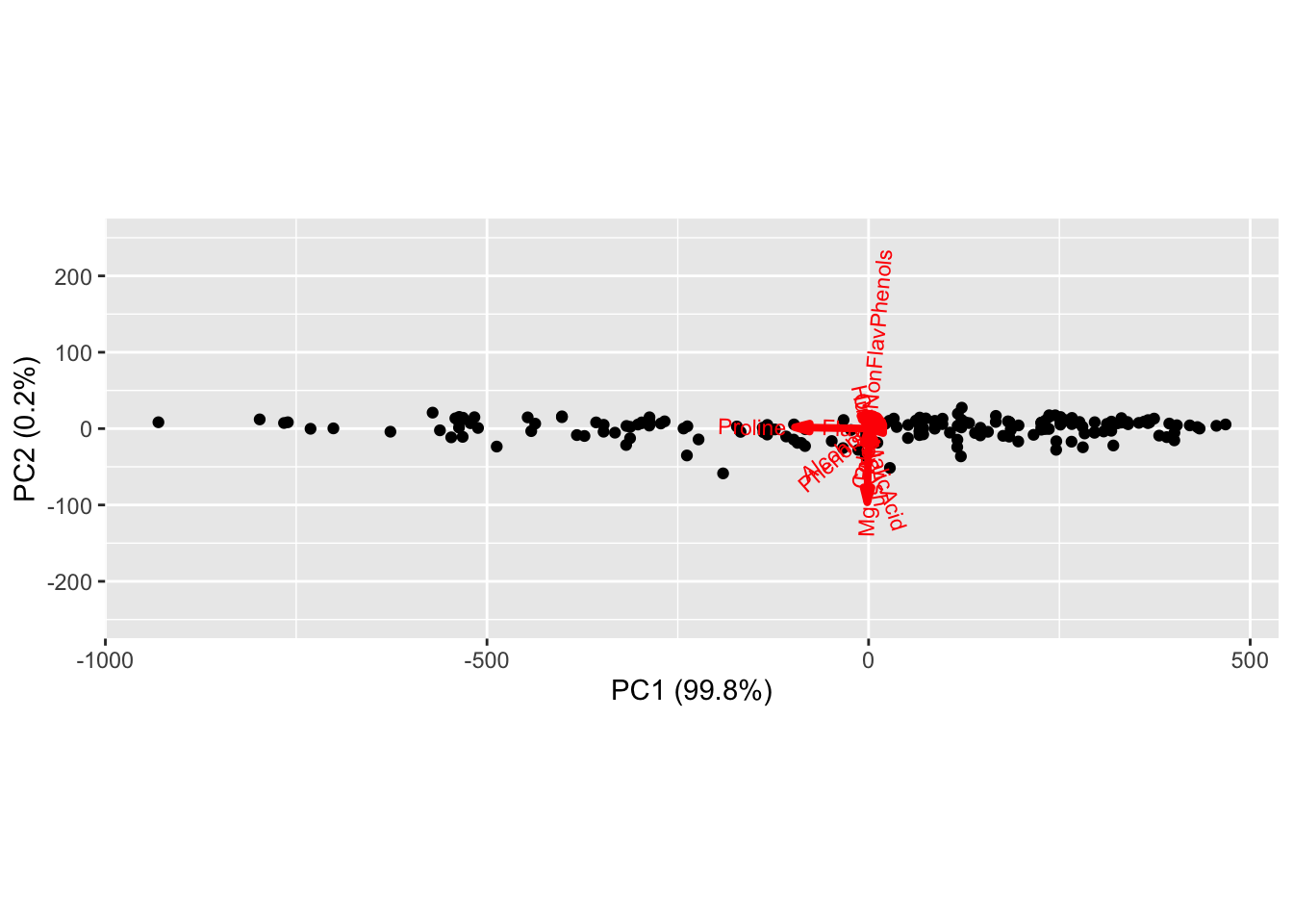
In the figure above, the black dots are scatterplots of the first and second principal component score for each sample in our data set, i.e. \(\{(y_{i1},y_{i2})\}_{i=1}^N\), whereas the arrows correspond to the contribution of each column of the data matrix to the first and second loadings, i.e. \(\{(\vec{w}_1)_j,(\vec{w}_2)_j\}_{j=1}^d\). The red vector associated with proline is the only one with a large horizontal component, indicating it is essentially the only coordinate contributing to the first loading. A similar observation indicates magnesium is the only coordinate contributing to the second loading. Admittedly, the arrow corresponding to the variables are difficult to see, but we can zoom in closer to the origin where the results are clear.
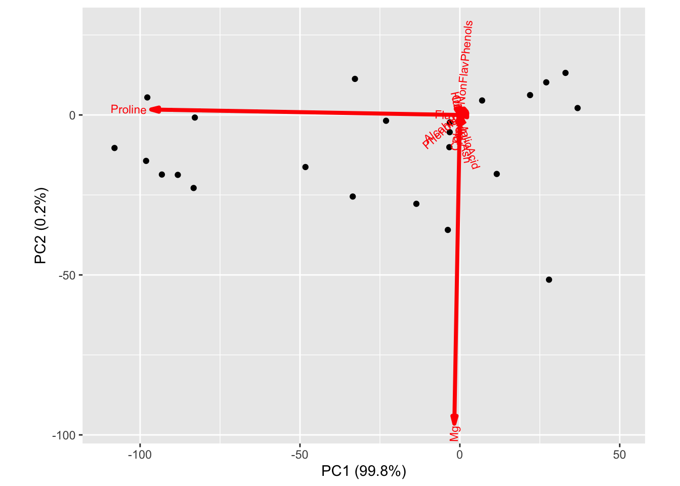
A natural way (and generally good idea) to address this issue is to standardize the columns of the data matrix prior to running PCA. If we use this approach for the wine data, we get the following biplot where there is much more diverse contributions to the first and second loadings from many coordinates.
 ##### Outliers
The existence of an outlier in a dataset (as in the univariate case) will alter the calculation of a sample covariance. However, a point can be an outlier because it has an extreme value in one or more of its coordinates. Unfortunately, standardization will not do much to alter this issue. Nonethess, the biplot is a helpful method for identifying this issue. Consider the wine data set, but let us now append a new data vector. It has the same values as the first row, except let’s set the malic acid and ash columns to \(10^6\) (these are unrealistic extreme values only intended to emphasis the effect of an outlier). Below we show the scree plot and biplot resulting from PCA without standardization.

Figure 4.6: PCA on wine data with an outlier
Here, we see one point has an extreme PC score associated with the outlier, which also accounts for a single large variance. It would be inappropriate to assume that a single PC component is sufficient to describe the data. Additionally, observe that the first loading is dominated by Malic Acid and Ash, values for which the outlier is extreme. Standardizing the coordinates can reduce the impact of the outlier but cannot remove it entirely. In such as case, further investigation to see the specific impact the outlier has on the loadings (and the potential overemphasis on some features) warrants further investigation.
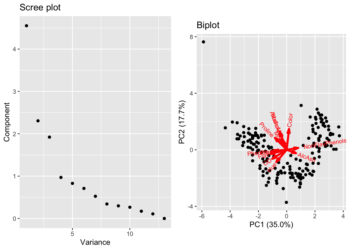
Figure 4.7: PCA on wine data with outlier after standardization
4.1.2.2.2 Nonlinear structure
Approximations using PCA are built via linear combinations of the loadings. However, there is not reason to a priori expect that the lower dimensional structure of our data is inherently linear. As such, PCA (and the other linear methods we’ll discuss in the remainder of this chapter) are limited in the complexity of structure they can discover in data. As a final example, consider the following data on a curve in \(\mathbb{R}^3\).
These data reside on a one-dimensional curve, specifically the curve parameterized by the equation \[t \mapsto (t\cos(t),t\sin(t),t^2/20)^T.\]
However, if we inspect the principal component variance, we do not see a clear separation in the first PC variance with the second and third. There is a jump between the second and third, and plotting the first two scores (biplot) shows the nonlinear structure.
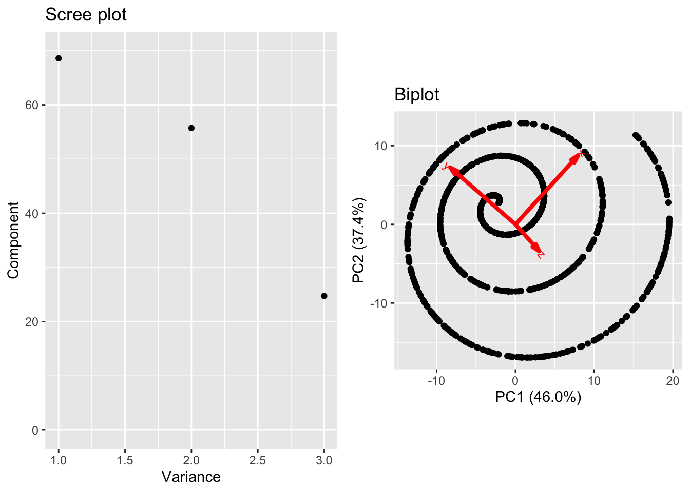
Ultimately, the fundamental limitation of PCA is a direct byproduct of it’s primary strength. PCA discovers best approximating hyperplanes but nothing more complex!
4.2 Singular Value Decomposition
4.2.1 Low-rank approximations
In the next two subsections, we are going to focus on low-rank matrix approximation methods in which we try to approximate our data matrix \({\bf X}\) using a low-rank alternative. In the language of dimension reduction, the idea is to approximate each data with a linear combination of a small number (\(k< d\) of latent feature vectors. Briefly, let’s discuss how this idea works in the case of PCA.
In PCA, the loadings provide a data-driven orthonormal basis \(\vec{w}_1,\dots,\vec{w}_d\) which allow us to compute the PCA scores from the centered data. In matrix notation, this scores are given by \[\underbrace{{\bf Y}}_{\text{PCA scores}} = \underbrace{({\bf HX})}_{\text{centered data matrix}} \times \underbrace{{\bf W}}_{\text{loadings}}.\]
The matrix \({\bf W}\) is orthonormal allowing us to write \[{\bf HX} = {\bf YW }^T.\] The \(ith\) row of the preceding matrix equality reads \[(\vec{x}_i - \bar{x})^T = \sum_{j=1}^d {\bf Y}_{ij} \vec{w}_j^T.\] From the PCA notes, an approximation using the first \(k\) loadings \[(\vec{x}_i - \bar{x})^T \approx \sum_{j=1}^k {\bf Y}_{ij} \vec{w}_j^T\] minimizes the average squared Euclidean distance over all vectors. In matrix notation, the approximation over all vectors decomposes as the product of an \(N\times k\) matrix and a \(k\times d\) matrix as follows. \[{\bf HX} \approx \underbrace{\begin{bmatrix}{\bf Y}_{11} & \dots & {\bf Y}_{1k} \\ \vdots & & \vdots \\ \vdots & & \vdots \\ {\bf Y}_{N1} & \dots & {\bf Y}_{Nk}\end{bmatrix}}_{N\times k} \underbrace{\begin{bmatrix}\vec{w}_1^T \\ \vdots \\ \vec{w}_k^T \vphantom{\vdots} \end{bmatrix}\\}_{k\times d}.\]
Due to the properties of the scores and loadings, the approximation is a rank \(k\) matrix. In the following sections, we’ll seek similar decompositions of our data matrix.
4.2.2 SVD and Low Rank Approximations
The standard problem for low rank matrix approximations is to solve the following problem. Given a matrix \({\bf X}\in\mathbb{R}^{N\times d}\) and a chosen rank \(k\), we want: \[ \text{argmin}_{{\bf Z}\in\mathbb{R}^{N\times d}} \|{\bf X} - {\bf Z}\|_F^2 = \] subject to the constraint that \({\bf Z}\) has rank \(k\).
Solving this constrained minimization problem may appear difficult, but the answer is obtainable directly from the SVD of \({\bf X}\) due to the following theorem.
Theorem 4.3 (Eckart-Young-Mirsky Theorem) Suppose matrix \({\bf X}\in\mathbb{R}^{N\times d}\) has singular value decomposition \[{\bf X} = {\bf US V}^T\] with singular values \[\sigma_1\ge\dots \ge \sigma_{\min\{N,d\}}.\] Then 1) For any rank \(k\) matrix \({\bf Z}\in\mathbb{R}^{N\times d}\), \[\|{\bf X}-{\bf Z}\|_F^2 \ge \sigma_{k+1}^2 + \dots + \sigma_{\min\{N,d\}}^2\] 2) The rank \(k\) matrix attained by keeping the first \(k\) left singular vectors, right singular vectors, and singular values of the SVD of \({\bf X}\) attains this minimum. Specifically, if \(\vec{u}_1,\dots,\vec{u}_k\) are the first \(k\) left singular vectors and \(\vec{v}_1,\dots,\vec{v}_k\) are the first \(k\) right singular vectors then \[\tilde{X} = \sum_{j=1}^k \sigma_j \vec{u}_j\vec{v}_j^T\] is the best rank \(k\) approximation to \({\bf X}\) under (squared) Frobenius loss.
There are several important implications of this theorem. First, the direct result indicates that computing the SVD of \({\bf X}\) immediately allows us to compute the best approximation under Frobenius loss for a specified rank \(k\). In practice, the full SVD is not required since we will typically consider the case where \(k <\min\{N,d\}\). There is a another implication as well. In cases where a specific choice of \(k\) is not clear, the singular values of \({\bf X}\) provide a method to comparing different choices of \(k\). Akin to the scree plot, we can plot the (squared) singular values to look for clear separation or alternatively, plot the ratio \[\frac{\sum_{j=1}^k\sigma_j^2}{\sum_{j=1}^{\min\{N,d\}}\sigma_j^2}\] as a function of \(k\) to understand the relative error for a specific choice of \(k\).
For a given choice of \(k\), we now approximate our original data by linear combination of the right singular vectors \(\vec{v}_1,\dots,\vec{v}_k\). The approximations are \[\vec{x}_i \approx \vec{z}_i = \sum_{j=1}^k \sigma_j{\bf U}_{ij} \vec{v}_j\].
4.2.3 Connections with PCA
Suppose that we were to compute the full SVD of the centered data matrix \[{\bf HX}= {\bf USV}^T.\] We can express the sample covariance matrix of the original data using the SVD as \[\begin{equation} \hat{\Sigma}_X = \frac{1}{N} ({\bf HX})^T ({\bf HX}) = \frac{1}{N} {\bf VS}^T{\bf U}^T{\bf U SV} ^T = {\bf V}\left(\frac{1}{N} {\bf S}^T{\bf S}\right) {\bf V}^T. \end{equation}\] The matrix \(\frac{1}{N}{\bf S}^T {\bf S} \in \mathbb{R}^{d\times d}\) is diagonal with entries \(\sigma_1^2/N \ge \dots \ge \sigma_d^2/N.\) Furthermore, the matrix \({\bf V}\) is orthonormal. Thus, from the SVD of \({\bf HX}\) we can immediately compute the spectral decomposition of \(\hat{\Sigma}_X\) to attain the principal component variances and loadings. In fact, the principal component loadings are the right singular vectors of \({\bf HX}\) whereas the principal component variances are the squared singular values divided by \(N\), e.g. \(\lambda_j = \sigma_j^2/N\). Using this observation, \[{\bf HX} = {\bf USV}^T \rightarrow {\bf HXV} = {\bf US}\] from which we may conclude the principal component scores are equal to \({\bf US}.\) This connection is the basis for most numerical implementation of PCA since it is more both faster and more numerically stable to compute the SVD of \({\bf HX}\) than to compute both \(\hat{\Sigma}_X\) and its eigendecomposition! Thus, computing the best rank \(k\) approximation to a centered data matrix is equivalent to the best approximation of the centered data using the first \(k\) PC scores.
However, using the SVD to compute a low rank approximation to a non-centered data matrix will give a different result than PCA since the SVD of \({\bf HX}\) will be different than the SVD of \({\bf X}\). Unlike PCA, which decomposes variability in directions relative to the center of the data, SVD learns an orthonormal basis which decomposes variability relative to the origin. Only when the data is centered (so its mean is the origin) do SVD and PCA coincide. Nonetheless, SVD has similar weaknesses to PCA including a sensitivity to scaling and outliers and an inability to detect nonlinear structure.
SVD can provide one final note of insight regarding PCA. Suppose that \(N < d\), which is to say that we have fewer samples than the dimensionality of our data. After centering, the matrix \({\bf HX}\) will have rank most \(N-1\). (Centering reduces the maximum possible rank from \(N\) to \(N-1\)). The SVD of \({\bf HX}\) will have at most \(d-1\) non-zero singular values. Thus, \(\hat{\Sigma}_X\) will have at most \(N-1\) non-zero PC variances and we can conclude that our data reside on a hyperplane of dimension \(N-1\) (possibly lower if \({\bf HX}\) has rank less than \(N-1\)). Since \(N-1 < d\), we are guaranteed to find a lower-dimensional representation of our data! However, this conclusion should be viewed cautiously. Should additional samples be drawn, can we conclude that they would also be constrained to the same hyperplane learned using the first \(N\) samples?
4.2.4 Recommender Systems
SVD may also be applied to association rule learning which can identify similar items in a datasets based on partial observations. As a motivating example, consider the case where we have a dataset of user provided ratings of products, which could be items purchased, songs listed to, or movies watched. In this case, \({\bf X}_{ij}\) indicates user \(i\)s rating of item \(j\). Typically, most of the entries of \({\bf X}\) will be NA since users have likely interacted with a small number of items. Using a variant of SVD, a simple recommendation system proceeds in two steps. First, we can impute the missing ratings. We can then use this result to infer similar movies which can be used for recommendation.
4.2.4.1 Imputation
Let \({\bf X}\in\mathbb{R}^{N\times d}\) be the data matrix of user ratings with rows corresponding to user and columns to items and \[\mathcal{I} =\{ij \, \text{ s.t. } {\bf X}_{ij} \ne NA\}\] be the set of all indices of \({\bf X}\) for which we have observed ratings. For any approximating matrix \(\tilde{\bf X}\in\mathbb{R}^{N\times d}\), we may define a `Frobenius’-like error as \[\mathbb{L}({\bf X},\tilde{\bf X}) = \sum_{ij \in \mathcal{I}} ({\bf X}_{ij}-\tilde{\bf X}_{ij})^2\] which is the sum-squared error over all observations. Using this definition of loss, here’s a simple algorithm for imputing the missing entries of \({\bf X}\) using low rank approximations of a pre-specified rank \(k\).
We initialize the matrix \(\tilde{\bf X}\) of imputed entries by taking \[\tilde{X}_{ij}= \begin{cases} X_{ij} & ij \in \mathcal{I} \\ 0 & ij \ne \mathcal{I} \end{cases}.\] Now let’s use the SVD of \(\tilde{\bf X}\) to compute a rank \(k\) approximation, \({\bf X}^{(k)}\). Update our imputed matrix \(\tilde{\bf X}= \tilde{\bf X}^{(k)}\) and compute the error \[\ell = \mathbb{L}({\bf X},\tilde{\bf X})\]. The low-rank approximation will distort all entries of \(\tilde{\bf X}\) so that \(\ell > 0\). We now repeat the following two steps.
Overwrite the entries of \(\tilde{\bf X}\) corresponding to observations in \({\bf X}\), e.g. for all \(ij \in \mathcal{I}\), set \(\tilde{\bf X}_{ij} = {\bf X}_{ij}\). The entries corresponding to missing observations generated by the low-rank approximation are kept unchanged. Now recompute the SVD of \(\tilde{\bf X}\) to find the rank \(k\) approximating matrix \(\tilde{\bf X}^{(k)}\). Update our imputed matrix using the low-rank approximation so that \(\tilde{\bf X} = {\bf X}^{(k)}\) and recompute the error \(\ell^* = \mathbb{L}({\bf X},\tilde{\bf X}).\)
If \(\ell^* < \ell\) and \(|\ell - \ell^*|/\ell > \epsilon\) then set \(\ell = \ell^*\) and return to step (1). Else stop the algorithm and we use matrix \(\tilde{\bf X}\) as our matrix of imputed values.
In summary, after initialization, we are continually overwriting the entries of our matrix of imputed values corresponding to observations then applyin a low-rank approximation. We stop the algorithm when the error stops decreasing or when the relative decrease in error is less than a specified threshhold \(\epsilon.\) In addition to the rank \(k\) and the stopping threshhold \(\epsilon\) there is one other important `tuning’ parameter, the initialization. In the brief description above, we used a standard of 0, but one could also use the average of all entries in the corresponding column (average item rating) or row (average rating given by a user) or some other specification. Many more complicated recommendation systems include user and item specific initializations and adjustments but still imploy a low rank approximation somewhere in their deployment.
In later updates, we show an application of this algorithm to the Movielens 10m dataset containing 10 million ratings from 72,000 viewers for 10,000 movies. To handle the size of this dataset, we use the Fast Truncated Singular Value Decomposition.
# library("irlba")
# initialize <- function(mat){
# # get column means ignoring NAs
# ave.rat <- colMeans(mat,na.rm = TRUE)
# # fill NAs by average movie rating
# for(j in 1:ncol(mat)){
#   mat[is.na(mat[,j]),j] <- ave.rat[j]
# }
# return(mat)
# }
#
# maxim <- function(mat,k){
# # temp <- svd(mat)
# temp<- irlba(mat, nv = k)
# return(list(U = temp$u[,1:k],
#             D = temp$d[1:k],
#             V = temp$v[,1:k],
#             mat.hat = temp$u[,1:k] %*% diag(temp$d[1:k]) %*% t(temp$v[,1:k])))
# }
#
# recommender <- function(mat, num_steps, k){
# # initialize loss function tracking
# loss <- rep(NA,num_steps)
# # run EM algorithm and save loss
# ind.known <- !is.na(mat)
# mat2 <- initialize(mat)
# for (j in 1:num_steps){
#   mat2 <- maxim(mat2,k)$mat.hat
#   loss[j] <- sum((mat2[ind.known] - mat[ind.known])^2)
#   mat2[ind.known] <- mat[ind.known]
# }
# return(list(loss= loss, fit = mat2))
# }
#
# k <- 3
# temp <- recommender(ratings,num_steps = 200, k = k)
# plot(temp$loss, xlab = "Step", ylab = expression(ell))
4.2.4.2 Recommendation
Suppose now that we have a matrix, \(\tilde{\bf X}\in\mathbb{R}^{N\times d}\) of movie ratings (real or imputed) and its SVD \[\tilde{\bf X} = \tilde{\bf U}\tilde{\bf S}\tilde{\bf V}^T\] where \(\tilde{\bf U} \in \mathbb{R}^{N\times k}\), \(\tilde{\bf S}\in\mathbb{R}^{k\times k}\) and \(\tilde{\bf V}\in\mathbb{R}^{d\times k}.\) Then for user \(i\) the rating they give to movie \(j\) is a linear combination of the elements in the \(j\) column of \(\tilde{\bf V}^T\). Specifically, \[\tilde{\bf X} \approx \sum_{\ell = 1}^k \sigma_\ell \tilde{\bf U}_{i\ell} (\tilde{\bf V})^T_{\ell j} = \sum_{\ell = 1}^k \sigma_\ell \tilde{\bf U}_{i\ell} \tilde{\bf V}_{j\ell}.\]
For any movie, its rating will always be a linear combination of the elements in the corresponding column of \(\tilde{V}^T\). As such, we may view the \(k\)-dimensional vectors in each column of \(\tilde{\bf V}\) as a representation of that movie. We may then use these vectors to identify similar movies; one common approach is the cosine similarity, which for vectors \(\vec{x}, \vec{y}\in\mathbb{R}^k\) is the cosine of the angle between them, i.e. \[\cos\theta = \frac{\vec{x}^T\vec{y}}{\|\vec{x}\| \|\vec{y}\|}.\] The cosine similarity is bounded between -1 and 1 and two vectors are considered more similar if the cosine of the angle between them is closer to 1. Using this representation, we can take any movie (a column of \(\tilde{\bf V}^T\)) and choose the most similar movie (choosing the other columns of \(\tilde{\bf V}^T\) with the largest cosine similarity). Thus, if a user gave a high rating to movie \(b\), we now have a method for recommending one or more similar movies they might enjoy.
4.3 Nonnegative Matrix Factorization
In both PCA and SVD, we learn data-driven orthonormal feature vectors which we can use to decompose our data in an orderly fashion. Nonnegative matrix factorization (NMF) is again focused on learning a set latent vectors which can be used to approximate our data. However, we will add a few restrictions motivated by experimental data and a desire to increase interpretability of the results which will drastically alter the results.
For NMF, we focus on cases where \({\bf X}\) is an \(N\times d\) data matrix with the added condition that its entries are nonnegative. Notationally, we write \({\bf X}\in\mathbb{R}_{\ge 0}^{N\times d}\) to indicate it is composed of nonnegative real values. The nonnegativity condition is a natural constraint for many experimental data sets, but we are also going to impose a similar constraint on our feature vectors and coefficients. More specifically, for a specific rank \(k\), we seek a coefficient matrix \({\bf W}\in\mathbb{R}_{\ge 0}^{N\times k}\) and feature matrix \({\bf H}\in \mathbb{R}^{k\times d}_{\ge 0}\) such that \({\bf WH}\) is as close to \({\bf X}\) as possible. The nonnegativity constraint on the elements of \({\bf W}\) and \({\bf H}\) implies that \({\bf WH}\in\mathbb{R}_{\ge 0}^{N\times d}\). There are many different measures of proximity that one may use in NMF which are greater than zero and equal to zero if and only if \({\bf X}={\bf WH}\). The most common measures are
Frobenius norm: \(\|{\bf X}-{\bf WH}\|_F.\)
Divergence: \(D({\bf X} \| {\bf WH}) = \sum_{i=1}^N\sum_{j=1}^d \left[{\bf X}_{ij} \log \frac{{\bf X}_{ij}}{({\bf WH})_{ij}} + ({\bf WH})_{ij} - {\bf X}_{ij}\right]\)
Itakura-Saito Divergence: \[D_{IS}({\bf X}, {\bf WH}) = \sum_{i=1}^N\sum_{j=1}^d \left[\frac{{\bf X}_{ij}}{({\bf WH})_{ij}} - \log\frac{{\bf X}_{ij}}{({\bf WH})_{ij}} -1 \right]\]
These loss functions emphasize and prioritize different features of the data and are often coupled with additional penalties or assumptions on the elements of \({\bf W}\) and \({\bf H}\) which we will discuss at the end of the section. From a statistical perspective, they may also be motivated based on differing beliefs about the data generating process. For example, suppose we assume conditional independence of the entries of \({\bf X}\) given \({\bf W}\), \({\bf H}\), and error variance \(\sigma\). Under a Gaussian error model \[{\bf X}_{ij} \mid {\bf W},\,{\bf H} \sim \mathcal{N}\left(({\bf WH})_{ij},\sigma^2\right)\] maximizing the associated likelihood w.r.t. \({\bf W}\) and \({\bf H}\) is equivalent to minimization of the Frobenius norm \(\|{\bf X}-{\bf WH}\|_F^2.\) We’ll revisit this idea in greater detail in Section 4.3.6.
For now, let us focus on the primary motivation of NMF, which is to create more interpretable feature vectors (the rows of \({\bf H}\)).
4.3.1 Interpretability, Superpositions, and Positive Spans
Consider the case of SVD where we can approximate a given vector \(\vec{x}_i\) using the first \(k\) right singular vectors as
\[\vec{x}_i \approx \sum_{j=1}^k \sigma_j {\bf U}_{ij} \vec{v}_j.\] Let us restrict ourselves to the case of nonnegative entries. Suppose for the moment that the \(\ell\)th coordinate of \(\vec{x}_i\) is (very close to) zero and this is reflected by our approximation as well so that \[(\vec{x}_i)_\ell \approx \sum_{j=1}^k \sigma_j {\bf U}_{ij} (\vec{v}_j)_\ell \approx 0.\]
The freedom of the coefficients \(\sigma_j {\bf U}_{ij}\) and the features \((\vec{v}_j)_\ell\) for \(j=1,\dots,k\) to take any value in \(\mathbb{R}\) prevents us from concluding that there is a comparable near-zeroness in the features or coefficients. In could be that case that \({\bf U}_{ij} (\vec{v}_j)_\ell\) is near zero for all \(j=1,\dots,k\) or that some subset are large and positive but are canceled out by a different subset that is large and negative. If, however, we restrict the coefficients and features to be zero this cancellation effect cannot occur. Features can only then be added but never subtracted. Under this restriction, \(\sum_{j=1}^k \sigma_j {\bf U}_{ij} (\vec{v}_j)_\ell\) will only be close to zero if the coefficients are (near) zero for any feature vector which has a (large) positive entry in its \(\ell\)th coordinate.
Thus, in a factorization of the form \[\vec{x}_i \approx \sum_{j=1}^k \underbrace{{\bf W}_{ij}}_{\ge 0} \underbrace{\vec{h}_j}_{\in \mathbb{R}^d_{\ge}},\] we can only superimpose (add) features to approximate our data, we might expect the features themselves to look more like our data. In matrix notation, we have \[{\bf X} = {\bf WH}\] where the coefficients for each sample are stored in the rows of \({\bf W}\in\mathbb{R}^{N\times k}_{\ge 0}\) and the features are transposed and listed as the rows of \({\bf H}\in\mathbb{R}^{k\times d}\).
4.3.2 Geometric Interpretation
As a motivating example consider the case, where we have data \(\vec{x}_1,\dots,\vec{x}_N\in\mathbb{R}^3_{\ge 0}\) for which there is a exact decomposition \[{\bf X} = {\bf WH}\] which is to say there are nonnegative coefficients, \({\bf W}\) and feature vectors \(\vec{h}_1,\vec{h}_2 \in \mathbb{R}_{\ge 0}^3\) such that \[\vec{x}_i = {\bf W}_{i1}\vec{h}_1 + {\bf W}_{i2}\vec{h}_2 \qquad \text{ for } i =1,\dots,N.\] The nonnegativity condition on data implies that \(\vec{x}_1,\dots,\vec{x}_N\) reside in the positive orthant of \(\mathbb{R}^3.\) The exact decomposition assumptions implies \(\{\vec{x}_1,\dots,\vec{x}_N\} \in \text{span}\{\vec{h}_1,\vec{h}_2\}\) and furthermore the following more restricted picture holds.Figure 4.8: Data in the positive span of two vectors
The data are constrained within the positive span of the vectors, a notion we may now define.
Definition 4.2 (Positive Span) The positive span of a set of vectors \(\{\vec{h}_1,\dots,\vec{h}_k\}\in\mathbb{R}^d\) is the set \[\Gamma\left(\{\vec{h}_1,\dots,\vec{h}_k\}\right) = \left\{\vec{v}\in\mathbb{R}^d \, \bigg|\, \vec{v} = \sum_{j=1}^k a_j \vec{h}_j, \, a_1,\dots,a_k \ge 0\right\}.\] This set is also called the simplicial cone or conical hull of \(\{\vec{h}_1,\dots,\vec{h}_k\}\).
In the motivating example above, our data live in the positive span of the two feature vectors, thus we say the data matrix \({\bf X}\) has a nonnegative matrix factorization \({\bf WH}\).
Thus, we may view NMF as a restricted version of PCA or SVD where we have moved from spans to positive spans. This seemingly small change gives rise to some big problems. Even in this simple case above we have a uniqueness problem. Up to sign changes and ordering, the feature vectors in PCA and SVD were unique. However, we can find two alternative vectors \(\vec{h}_1'\) and \(\vec{h}_2'\) which still give a exact NMF. There are trivial cases. First, one can change ordering (\(\vec{h}_1' =\vec{h}_2\) and \(\vec{h}_2' = \vec{h}_1\)) which we avoid in PCA and SVD by assuming the corresponding singular values of PC variances are listed in decreasaing order. Secondly, we could rescale by setting \(\vec{h}_1' = c\vec{h}_1\) and rescaling the corresponding coefficients by a factor of \(1/c\) for some \(c > 0\) which PCA and SVD avoid by fixing feature vectors to have unit length. The ordering issue is a labeling concern and may be ignored, whereas the rescaling issue can be addressed by adding constraints on the length of the feature vectors.
A third and far more subtle issue occurs because we do not enforce orthogonality. In @ref[fig:nmf-ex], imagine that the feature vectors are the arms of a folding fan. We could change the angle between our feature vectors by opening or closing the arms of the fan. So long as we do not close the fan too much (and leave our data outside the positive span) or open them too much (so that feature vectors have negative entries), we can still find a perfect reconstruction. This `folding fan’ issue can be addressed through additional penalties which we discuss in @ref{sec-nmf-ext}, but nonuniqueness cannot be eliminated entirely. Thus, we seek an NMF for our data rather than the NMF.
4.3.3 Finding a NMF: Multiplicative Updates
For a given choice of error, the lack of a unique solution also means there is no closed form solution for \({\bf W}\) and \({\bf H}\). Thus, we will need to apply numerical optimization to find a \({\bf W}\) and \({\bf H}\) which minimizes the selected error, \[\text{argmin}_{{\bf W}\in\mathbb{R}^{N\times k}_{\ge 0}, {\bf H}\in\mathbb{R}^{k\times d}_{\ge 0}}\,\,\,\,\, D({\bf X},{\bf WH})\]. The loss is a function of all of the entries of \({\bf W}\) and \({\bf H}\). To apply any type of gradient based optimization, we need to compute the partial derivative of our loss with respect to each of the entries of these matrices.
As an example, we will focus on the divergence and show the relevant details. For gradient based optimization, we then need to compute \(\frac{\partial }{\partial {\bf W}_{ij}} D({\bf X}\| {\bf WH})\) for \(`\le i \le N\) and \(1\le j\le k\) and \(\frac{\partial }{\partial {\bf H}_{j\ell}} D({\bf X}\| {\bf WH})\) for \(1\le j \le k\) and \(1\le \ell \le d.\) Note that \[({\bf WH})_{st} = \sum_{j=1}^k{\bf W}_{sk}{\bf H}_{kt}\] so that \[\frac{\partial ({\bf WH})_{st}}{\partial ({\bf WH})_{ij}} = \begin{cases} {\bf H}_{jt} & s = i \\ 0 & s\ne i \end{cases}\] Thus, we may may make use of the chain rule to conclude that \[\begin{align*} \frac{\partial }{\partial {\bf W}_{ij}} D({bf X}\| {\bf WH}) &= \frac{\partial }{\partial {\bf W}_{ij}}\sum_{st} \left({\bf X}_{st} \log(({\bf X})_{st}) - {\bf X}_{st} \log(({\bf WH})_{st}) + ({\bf WH})_st - ({\bf X})_{st}\right)\\ &=\frac{\partial }{\partial {\bf W}_{ij}}\sum_{st} \left(- {\bf X}_{st} \log(({\bf WH})_{st}) + ({\bf WH})_{st} \right) \\ &=\sum_{st}\left(\frac{{\bf X}_{st}}{({\bf WH}_{st})} + 1\right)\frac{\partial ({\bf WH})_{st}}{\partial {\bf W}_{ij}} \\ &=\sum_{t=1}^d \left(-\frac{{\bf X}_{it}}{({\bf WH}_{it})} + 1\right){\bf H}_{jt}. \end{align*}\] A similar calculation gives \[\frac{\partial }{\partial {\bf H}_{ij}} D({bf X}\| {\bf WH}) = \sum_{s=1}^N \left(-\frac{{\bf X}_{sj}}{({\bf WH})_{sj}} + 1\right) {\bf W}_{sj}.\] In a standard implementation of gradient descent, we choose a step size \(\epsilon >0\) and apply the updates \[\begin{equation} \begin{split} {\bf W}_{ij} \leftarrow {\bf W}_{ij} - \epsilon \sum_{t=1}^d \left(-\frac{{\bf X}_{it}}{({\bf WH}_{it})} + 1\right){\bf H}_{jt} \\ {\bf H}_{ij} \leftarrow {\bf H}_{ij} - \epsilon \sum_{s=1}^N \left(-\frac{{\bf X}_{sj}}{({\bf WH})_{sj}} + 1\right) {\bf W}_{sj} \end{split} \end{equation}\] to each entry of \({\bf W}\) and \({\bf H}\) simultaneously. Alternatively, we could consider coordinate descent where we update each entry of \({\bf W}\) (holding all other entries of \({\bf W}\) and \({\bf H}\) constant) separately then do the same for \({\bf H}\) then repeat. Each approach will converge to a local mode (though possibly different ones) when \(\epsilon\) is sufficiently small. However, if \(\epsilon\) is too small it may take many iterations to converge. Unfortunately, choosing \(\epsilon\) can create a numerically unstable algorithm (that doesn’t converge at all) or one where we lose the nonnegativity condition on the entries of \({\bf W}\) or \({\bf H}\).
To preserve nonnegativity, [10] developed a set of state dependent step-sizes (one for each entry of \({\bf W}\) and \({\bf H}\)) which result in multiplicative rather than additive updates. For divergence, they take step sizes \[\epsilon_{ij}^{W} = \frac{{\bf W}_{ij}}{\sum_t {\bf H}_{jt}} \text{ and } \epsilon_{ij}^H = \frac{{\bf H}_{ij}}{\sum_s {\bf W}_{sj}}.\] These step size are proportional to the entries we are updating so that we take larger steps for larger entries of \({\bf W}\) of \({\bf H}\). If we substitute these step sizes in the updates simplify to
\[\begin{equation} \begin{split} {\bf W}_{ij} &\leftarrow {\bf W}_{ij} \left[\frac{\sum_t \left({\bf H}_{jt}{\bf X}_{it}/({\bf WH}_{it})\right)}{\sum_t {\bf H}_{jt}} \right] \\ {\bf H}_{ij} &\leftarrow {\bf H}_{ij} \left[\frac{\sum_s\left({\bf W}_{si}{\bf X_{sj}}/({\bf WH})_{si} \right)}{\sum_s {\bf W}_{si}}\right] \end{split} \end{equation}\]
indicating that we rescale the entries of \({\bf W}\) and \({\bf H}\) by some nonnegative value which is guaranteed to preserve the nonnegativity of each entry. A short proof showing convergence to a local mode may be found in the original paper by Lee and Seung along with multiplicative update rules for other choices of loss are also available in [10]. Deriving these updates are also provided as exercises for the reader. Furthermore, one can verify that the multiplicative updates simplify to one when \({\bf X}= {\bf WH}.\)
We can more compactly write the updates for each matrix using Hadamard notation, which gives the following multiplicative updates for \({\bf W}\) and \({\bf H}\)
\[\begin{equation} \begin{split} {\bf W} &\leftarrow {\bf W} \odot \left\{[{\bf X}\oslash( {\bf WH})]{\bf H}^T\right\} \oslash [{\bf 1}_{N\times d}{\bf H}^T] \\ {\bf H} &\leftarrow {\bf H} \odot \left\{{\bf W}^T [{\bf X} \oslash ({\bf WH})]\right\} \oslash [{\bf W}^T {\bf 1}_{N\times d} ] \end{split} \end{equation}\]
In most implementations of NMF, multiplicative updates for \({\bf W}\) and \({\bf H}\) are alternated until convergence. However, some packages also implement rescaling following each pair of multiplicative updates to enforce other constraints (such as sum to one constrains on the rows of \({\bf W}\) or columns of \({\bf H}\)). When using NMF it is good to check documentation to see if these additional steps are implemented.
4.3.4 NMF in practice
For a given choice of loss, standard NMF proceeds in the following manner.
- Choose a rank \(k\) and initial \({\bf W}_\in\mathbb{R}^{N\times k}_{\ge 0}\) and \({\bf H}\in\mathbb{R}^{k\times d}_{\ge 0}\).
- Apply the multiplicative rule until a local minimum is reached.
- Repeats steps (1) and (2) for different initial conditions then select the final \({\bf W}\) and \({\bf H}\) which give the lowest overall loss.
Different initial conditions (ICs) will converge to different local modes; reptition over multiple differents (ICs) will help find a better overall minimizer and avoid getting a final NMF which is trapped in a poor local mode. There is no guidance of how many ICs. Many packages default to five. More would be better but computational resources are not infinite, and finding even one mode though coordinate ascent can be slow. There are also methods based on nonnegativity constraints of the SVD (aptly named nonnegative SVD or NNSVD) for initialization which have shown good performance [11]. However, NNSVD initialization does increase computation burden.
The choice of \(k\) is also challenging. If prior information or other project constraints dictate a specific choice of \(k\) one should use that value. Alternatively, if visualization is a priority taking \(k=1,2,\) or \(3\) is a natural choice. Unfortunately, in many cases prior information is typically absent, thus data driven methods for selecting \(k\) from a range of possible choices are required. Importantly, since there are no connections between the rank \(k\) NMF and rank \(k+1\) NMF, one cannot truncate the vectors and coefficients and attain an optimal solution for a lower-dimensional representation as we can in PCA or SVD. Thus, separate fits at each choice of \(k\) must be attained through separate runs of the numerical optimization making NMF far more computationally demanding in practice.
Suppose for now, we have optimal NMF fits for a range of nonnegative ranks obtained by fitting separate NMF models for a range of ranks using multiple initial conditions or NNSVD based initialization at each rank. Given these fits, one natural approach is to follow a scree plot like approach similar to what we have used for PCA and NMF. One can then compare plot the loss as a function of \(k\) and look for an elbow where the error appears to saturate.
Much like SVD and PCA, unfortunately, there is often no clear elbow indicating an obvious choice of \(k\). As such, additional approaches have been suggested in the literature such as cross-validation where in the data is split into test-train sets and the robustness of loss is investigated at each rank. Bayesian methods for balancing low loss with model complexity (small \(k\)) are also viable but again rely on some prior on model complexity.Other authors have used connections between NMF and clustering to adapt methods for assessing the quality of (hierarchical) clustering to the case of finding an optimal \(k\) in NMF. For example, one can use the robustness (or lack thereof) of clustering of data at each rank measured by the cophenetic correlation to identify an optimal \(k\) [12]. We’ll discuss hierarchical clustering and the cophenetic correlation in more detail Chapter 7. For now, we’ll restate the advice from [12] and advocate for the value of \(k\) at which the cophenetic correlation begins to drop.
Example 4.2 (NMF applied to MNIST) As an example, we show NMF applied to the first \(100\) eights (to save computation time) from the MNIST dataset [1] using Divergence with five runs per rank. Below we fit separate NMFs for ranks 1 through 25 with 5 random initializations per fit. Divergence (residuals) and the cophenetic correlation are each shown below as a function of rank.
There is no clear elbow in the plot of the model residuals that clearly suggests an optimal rank between 1 and 25. The cophenetic correlation begins to drop after rank 2. Thus, the method of [12] suggests \(k=2\) is reasonable. In fact if we select a rank 2 NMF, we do get interpretable 8-like images as our feature images(vectors) which correspond to eights slanting in two different directions, a seemingly reasonable compression of structure in the data.
Compare this to the less 8-like images found using the features given by a rank 2 approximation from SVD.
4.3.5 Regularization and Interpretability
For a random initialization, the values of \({\bf W}\) and \({\bf H}\) obtained when the multiplicative rules are run to convergence not resemble the original data, which is contrary to our original goal of finding features which are more comparable to the data. More specifically, the feature vectors \(\vec{h}_1,\dots,\vec{h}_k\) which are superimposed to approximate the observations may appear quite different from the observations themselves. Many extensions of NMF address this issue through the inclusion of additional penalties on the elements of \({\bf W}\) or \({\bf H}\) which induce sparsity in the coefficients \({\bf W}\) and/or constrain the features to be more similar to the data. In practice, it is insufficient to apply penalties which depend solely on the scaling of either \({\bf W}\) or \({\bf H}\) as these can typically be made arbitrarily small by increasing corresponding elements of \({\bf H}\) or \({\bf W}\) respectively. Thus, any penalty which depends on the scaling of one matrix often includes additional constraints or penalties on the other.
Briefly, we discuss two version which are constructed to generate features which strongly mimic the original observations.
4.3.5.1 Archetypes
Before discussing Archetypal Analysis, we need an additional geometric idea.
Given a set of vectors \(\mathcal{H}=\{\vec{h}_1,\dots,\vec{h}_k\}\subset\mathbb{R}^d\), the convex hull of \(\mathcal{H}\) is the set \[\text{conv}(\mathcal{H}) = \{b_1\vec{h}_1+\cdots + b_k \vec{h}_k: b_1,\dots,b_k \ge 0,\, c_1+\dots+c_k = 1\}\]
The weights in the above definition are constrained to be positive, similar to the definition of positive span, but with the added constraint that they sum to one. Thus, for a set of vectors \(\mathcal{H}\)
\[\text{conv}(\mathcal{H}) \subset \Gamma(\mathcal{H}) \subset \text{span}(\mathcal{H}).\] An example of a convex hull (shown in grey) of set of vectors (points in red) in \(\mathbb{R}^2\) is shown below. Imagine wrapping a string around the set of points and pulling it tight. Everything on/within the loop is in the convex hull. An analogous interpretation holds in higher dimensions using a “sheet” rather than a string.
Importantly, we can view the coefficient \(c_1,\dots,c_k\) as defining (probability) weights. Thus, every point in the convex hull of \({\bf H}\) is a weighted average of the vectors in \(\mathcal{H}\) and one then expects any point in the convex hull of \(\mathcal{H}\) to resemble the vectors in \(\mathcal{H}\). In archetypal analysis [13], we add the constraint that the features (row of \({\bf H}\)) are themselves elements in the convex hull of the original data so that \({\bf H}= {\bf B X}\) where \({\bf B}\in\mathbb{R}_{\ge 0}^{k\times N}\) must satisfy the constraint \({\bf B}\vec{1}_N = \vec{1}_k\).
Under this setup, we then want to solve the following constrained optimization problem \[\text{argmin}_{{\bf W}\in \mathbb{R}_{\ge 0}^{N\times k},\,{\bf B}\in\mathbb{R}_{\ge 0}^{k\times N}, {\bf B}\vec{1}_N = \vec{1}_k}\| {\bf X}- {\bf WBX}\|_F.\]
The rows of \({\bf BX}\), called archetypes, reside are typically extremal in the sense that they reside on the boundary of the convex hull of the data. We show them below for a rank two approximation to the eights consistent with the choice in the example above.
4.3.5.2 Volume Regularized NMF
Much like Archetype Analysis, Volume regularized NMF creates feature vectors which resemble the observation through a more geometric approach [15]. Suppose that we are seeking a rank \(k\) approximation of data in \(d\) dimensions with \(k<d\). If the vectors \(\vec{h}_1,\dots,\vec{h}_k\) are affinely independent, i.e. they don’t live on a hyperplane of dimension less than \(k\), then the volume of the convex of hall of the vectors is given by the following formula \[\text{vol}\left(\text{conv}(\{\vec{h}_1,\dots,\vec{h}_k\})\right) = \frac{\sqrt{\text{det}(\tilde{\bf H}\tilde{\bf H}^T})}{(k-1)!}\] where \[\tilde{\bf H} = \begin{bmatrix} \vec{h}_1^T-\vec{h}_k^T \\ \vdots \\ \vec{h}_{k-1}^T-\vec{h}_k^T\end{bmatrix} \in \mathbb{R}^{(k-1)\times d}.\] An extension of this result is that for linearly independent vectors \(\vec{h}_1,\dots,\vec{h}_k\), the volume of the convex hull of the vectors \(\vec{0},\vec{h}_1,\dots,\vec{h}_k\) can be computed directly from our feature matrix \({\bf H}\), i.e. \[\text{vol}\left(\text{conv}(\{0,\vec{h}_1,\dots,\vec{h}_k\})\right) = \frac{\sqrt{\det({\bf H}{\bf H}^T})}{k!}.\]
One brief aside on the notion of volume here that is not typically made clear in the related literature. When \(k < d\), the convex hull of \(\vec{0},\vec{h}_1,\dots,\vec{h}_k\) is contained in a \(k\)-dimensional hyperplane. Thus, its \(d\)-dimensional volume must be zero. When we talk of the volume of a convex hull, we instead mean its \(k\)-dimensional volume. As an example, consider the case of a single vector \(\vec{h}_1\) in \(\mathbb{R}^3.\) The convex hull of \(\vec{0},\vec{h_1}\) is the line segment from the origin to \(\vec{h}_1\). Line segments have zero 3-dimensional volume, but they do have length (1-dimensional volume). In this case, the 1-dimensional volume of the convex hull is the length of the line segment, e.g. \(\|\vec{h}_1\|\).
Incorporating a penalty on the volume of the convex hull of the feature vectors gives rise to the aptly named volume-regularized NMF \[\text{argmin}_{{\bf W}_\in\mathbb{R}_{\ge 0}^{N\times k},{\bf W}\vec{1}_N = \vec{1}_k, {\bf H}\in \mathbb{R}_{\ge 0}^{k\times d}}\quad \|{\bf X}-{\bf WH}\|_F^2 + \lambda \sqrt{\text{det}({\bf HH}^T)}\] here the constraint \({\bf W}\vec{1}_N = \vec{1}_k\) requiring that the rows of \({\bf W}\) sum to one prevents an arbitrary shrinkage of the feature vectors towards zero. In some numerical implementation, this constraint is relaxed so that the sum of the rows of \({\bf W}\) are bounded above by one. The value \(\lambda\) is tuning parameter that must be specified by the user to balance goodness of fit vs minimal volume. Below we show the results of volume regularized NMF applied to the subset of the eights data studied above which strongly resemble results from the standard NMF implementation. However, this method was far more computationally efficient. Only one run of the VR-NMF was required, and it converged much more quickly than the vanilla NMF.
4.3.6 NMF and Maximum Likelihood Estimation
Throughout this section we have focused on the geometric aspects of NMF, but there are parallel statistical perspectives based on maximum likelihood estimation. For example, consider the model \[{\bf X}_{ij} \mid ({\bf WH}_{ij}) \sim \mathcal{N}\left(({\bf WH}_{ij},\sigma^2\right), \qquad 1\le i\le N, 1\le j\le d\] with the additional assumption that the observations in \({\bf X}\) are conditionally independent given \({\bf WH}\in \mathbb{R}^{N\times k}_{\ge 0}\), \({\bf H}\in\mathbb{R}^{k\times d}_\ge 0\) and \(\sigma\). Under this framework the likelihood of the data is then \[\mathcal{L}({\bf X}\mid{\bf WH}) \propto \frac{1}{\sqrt{2\pi\sigma^2}}\prod_{i=1}^N\prod_{j=1}^d \exp\left(-\frac{({\bf X}_{ij}-({\bf WH}_{ij}))^2}{\sigma^2}\right)\] which has log-likelihood \[\log \mathcal{L}({\bf X}\mid{\bf WH}) = -\frac{N}{2}\log\sigma^2-\frac{1}{\sigma^2}\sum_{i=1}^N\sum_{j=1}^d ({\bf X}_{ij}-({\bf WH}_{ij}))^2 = - \frac{N}{2}\log\sigma^2 -\frac{1}{\sigma^2}\|{\bf X}-{\bf WH}\|_F^2.\] Thus, minimizing the Frobenius norm is equivalent to maximizing the likelihood in this normal model with homoskedastic errors.
Similarly, divergence arises from a Poisson model \[{\bf X}_{ij} \mid ({\bf WH})_{ij} \sim \text{Pois}\left(({\bf WH})_{ij}\right)\] again with a low rank structure for \({\bf W}\) and \({\bf H}\) and the conditional independence assumption on the entries of \({\bf X}\) given \({\bf WH}\).
The IS divergence again uses conditional independence and a low rank structure for \({\bf WH}\) under the assumption of multiplicative Gamma distributed errors with mean one, i.e. \[{\bf X}_{ij} \mid ({\bf WH})_{ij} = ({\bf WH})_{ij} e_{ij}, \qquad\, e_{ij} \sim_{iid} \text{Gamma}(\alpha,\beta)\] with \(\alpha/\beta = 1\). See [16] for additional details.
4.4 Multidimensional Scaling
Multidimensional scaling (MDS) is a broad name for a myriad of different methods which are designed to handle a common problem. Suppose there are \(N\) objects of interest in a dataset. Examples include a set of geographic locations or cells from mass spectrometry or census blocks, etc. Importantly, we do not need actual data corresponding to each object. In MDS, we instead require a measure the distance or dissimilarity between each pair of objects. We can organize these distances into a matrix \({\bf \Delta}\in\mathbb{R}^{N\times N}\), with \({\bf \Delta}_{rs}\) representing the distance/dissimilarity between objects \(r\) and \(s\). Thus, \({\bf \Delta}_{rr}=0\) and for now, we may assume that \({\bf \Delta}_{sr} = {\bf \Delta}_{rs}\). The matrix \({\bf \Delta}\) is often called a Distance or Dissimilarity matrix. In practice, we may construct a distance matrix from observations, but for the purposes of MDS we only require \({\bf \Delta}\).
The primary goal of MDS is to find a set of lower-dimensional points \(\vec{y}_1, \dots, \vec{y}_N \in \mathbb{R}^{t}\) corresponding to each of the \(N\) objects such that the distance between \(\vec{y}_r\) and \(\vec{y}_s\) is close to \({\bf \Delta}_{rs}\). There are numerous different notions of distance one use in \(\mathbb{R}^t\). Additionally, we may not know the notion of distance/dissimilarity used when computing \({\bf \Delta}\) or if the dissimilarity corresponds to any well defined notion of distance. Euclidean distance is a common choice for the distance of the lower-dimensional vectors. Fixing this choice still leaves many open questions. Are the original distances Euclidean? If so, can we determine the dimensionality of the original data?
MDS also serves as a data visualization method. In this case, \(t\) is typically chosen to be either two or three, and the \(N\) points in the two-dimensional (or three-dimensional) representation may be plotted so that one can visualize the relationships between data. Before turning to the most common methods of MDS, let’s view a few examples using distances between cities.
Example 4.3 (Classical scaling applied to distances between cities) The eurodist R package provides air travel distances between 21 cities in Europe and 10 cities in the US. For the moment, we will focus on the 10 US cities with names and distances given in the following tables
## Found more than one class "dist" in cache; using the first, from namespace 'BiocGenerics'## Also defined by 'spam'## Found more than one class "dist" in cache; using the first, from namespace 'BiocGenerics'## Also defined by 'spam'| Atlanta | Chicago | Denver | Houston | LosAngeles | Miami | NewYork | SanFrancisco | Seattle | Washington.DC | |
|---|---|---|---|---|---|---|---|---|---|---|
| Atlanta | 0 | 587 | 1212 | 701 | 1936 | 604 | 748 | 2139 | 2182 | 543 |
| Chicago | 587 | 0 | 920 | 940 | 1745 | 1188 | 713 | 1858 | 1737 | 597 |
| Denver | 1212 | 920 | 0 | 879 | 831 | 1726 | 1631 | 949 | 1021 | 1494 |
| Houston | 701 | 940 | 879 | 0 | 1374 | 968 | 1420 | 1645 | 1891 | 1220 |
| LosAngeles | 1936 | 1745 | 831 | 1374 | 0 | 2339 | 2451 | 347 | 959 | 2300 |
| Miami | 604 | 1188 | 1726 | 968 | 2339 | 0 | 1092 | 2594 | 2734 | 923 |
| NewYork | 748 | 713 | 1631 | 1420 | 2451 | 1092 | 0 | 2571 | 2408 | 205 |
| SanFrancisco | 2139 | 1858 | 949 | 1645 | 347 | 2594 | 2571 | 0 | 678 | 2442 |
| Seattle | 2182 | 1737 | 1021 | 1891 | 959 | 2734 | 2408 | 678 | 0 | 2329 |
| Washington.DC | 543 | 597 | 1494 | 1220 | 2300 | 923 | 205 | 2442 | 2329 | 0 |
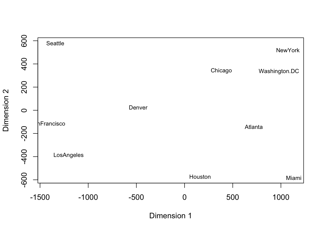
After conducting classical scaling (a method of MDS, details will be discussed later), we acquire the plot below. The plot is consistent with the geographical relationships between the cities. Miami and Seattle are the farthest apart in our plot. NY and D.C. are quite close on the plot, which is also true for Los Angeles and San Francisco.
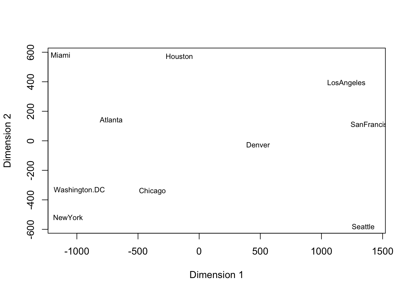
If we rotate the above plot 180 degrees, we recover an representation of the cities consistent with the typical map of the US.
Now let’s try MDS on the 21 European cities
| Athens | Barcelona | Brussels | Calais | Cherbourg | Cologne | Copenhagen | Geneva | Gibraltar | Hamburg | Hook of Holland | Lisbon | Lyons | Madrid | Marseilles | Milan | Munich | Paris | Rome | Stockholm | Vienna | |
|---|---|---|---|---|---|---|---|---|---|---|---|---|---|---|---|---|---|---|---|---|---|
| Athens | 0 | 3313 | 2963 | 3175 | 3339 | 2762 | 3276 | 2610 | 4485 | 2977 | 3030 | 4532 | 2753 | 3949 | 2865 | 2282 | 2179 | 3000 | 817 | 3927 | 1991 |
| Barcelona | 3313 | 0 | 1318 | 1326 | 1294 | 1498 | 2218 | 803 | 1172 | 2018 | 1490 | 1305 | 645 | 636 | 521 | 1014 | 1365 | 1033 | 1460 | 2868 | 1802 |
| Brussels | 2963 | 1318 | 0 | 204 | 583 | 206 | 966 | 677 | 2256 | 597 | 172 | 2084 | 690 | 1558 | 1011 | 925 | 747 | 285 | 1511 | 1616 | 1175 |
| Calais | 3175 | 1326 | 204 | 0 | 460 | 409 | 1136 | 747 | 2224 | 714 | 330 | 2052 | 739 | 1550 | 1059 | 1077 | 977 | 280 | 1662 | 1786 | 1381 |
| Cherbourg | 3339 | 1294 | 583 | 460 | 0 | 785 | 1545 | 853 | 2047 | 1115 | 731 | 1827 | 789 | 1347 | 1101 | 1209 | 1160 | 340 | 1794 | 2196 | 1588 |
| Cologne | 2762 | 1498 | 206 | 409 | 785 | 0 | 760 | 1662 | 2436 | 460 | 269 | 2290 | 714 | 1764 | 1035 | 911 | 583 | 465 | 1497 | 1403 | 937 |
| Copenhagen | 3276 | 2218 | 966 | 1136 | 1545 | 760 | 0 | 1418 | 3196 | 460 | 269 | 2971 | 1458 | 2498 | 1778 | 1537 | 1104 | 1176 | 2050 | 650 | 1455 |
| Geneva | 2610 | 803 | 677 | 747 | 853 | 1662 | 1418 | 0 | 1975 | 1118 | 895 | 1936 | 158 | 1439 | 425 | 328 | 591 | 513 | 995 | 2068 | 1019 |
| Gibraltar | 4485 | 1172 | 2256 | 2224 | 2047 | 2436 | 3196 | 1975 | 0 | 2897 | 2428 | 676 | 1817 | 698 | 1693 | 2185 | 2565 | 1971 | 2631 | 3886 | 2974 |
| Hamburg | 2977 | 2018 | 597 | 714 | 1115 | 460 | 460 | 1118 | 2897 | 0 | 550 | 2671 | 1159 | 2198 | 1479 | 1238 | 805 | 877 | 1751 | 949 | 1155 |
| Hook of Holland | 3030 | 1490 | 172 | 330 | 731 | 269 | 269 | 895 | 2428 | 550 | 0 | 2280 | 863 | 1730 | 1183 | 1098 | 851 | 457 | 1683 | 1500 | 1205 |
| Lisbon | 4532 | 1305 | 2084 | 2052 | 1827 | 2290 | 2971 | 1936 | 676 | 2671 | 2280 | 0 | 1178 | 668 | 1762 | 2250 | 2507 | 1799 | 2700 | 3231 | 2937 |
| Lyons | 2753 | 645 | 690 | 739 | 789 | 714 | 1458 | 158 | 1817 | 1159 | 863 | 1178 | 0 | 1281 | 320 | 328 | 724 | 471 | 1048 | 2108 | 1157 |
| Madrid | 3949 | 636 | 1558 | 1550 | 1347 | 1764 | 2498 | 1439 | 698 | 2198 | 1730 | 668 | 1281 | 0 | 1157 | 1724 | 2010 | 1273 | 2097 | 3188 | 2409 |
| Marseilles | 2865 | 521 | 1011 | 1059 | 1101 | 1035 | 1778 | 425 | 1693 | 1479 | 1183 | 1762 | 320 | 1157 | 0 | 618 | 1109 | 792 | 1011 | 2428 | 1363 |
| Milan | 2282 | 1014 | 925 | 1077 | 1209 | 911 | 1537 | 328 | 2185 | 1238 | 1098 | 2250 | 328 | 1724 | 618 | 0 | 331 | 856 | 586 | 2187 | 898 |
| Munich | 2179 | 1365 | 747 | 977 | 1160 | 583 | 1104 | 591 | 2565 | 805 | 851 | 2507 | 724 | 2010 | 1109 | 331 | 0 | 821 | 946 | 1754 | 428 |
| Paris | 3000 | 1033 | 285 | 280 | 340 | 465 | 1176 | 513 | 1971 | 877 | 457 | 1799 | 471 | 1273 | 792 | 856 | 821 | 0 | 1476 | 1827 | 1249 |
| Rome | 817 | 1460 | 1511 | 1662 | 1794 | 1497 | 2050 | 995 | 2631 | 1751 | 1683 | 2700 | 1048 | 2097 | 1011 | 586 | 946 | 1476 | 0 | 2707 | 1209 |
| Stockholm | 3927 | 2868 | 1616 | 1786 | 2196 | 1403 | 650 | 2068 | 3886 | 949 | 1500 | 3231 | 2108 | 3188 | 2428 | 2187 | 1754 | 1827 | 2707 | 0 | 2105 |
| Vienna | 1991 | 1802 | 1175 | 1381 | 1588 | 937 | 1455 | 1019 | 2974 | 1155 | 1205 | 2937 | 1157 | 2409 | 1363 | 898 | 428 | 1249 | 1209 | 2105 | 0 |
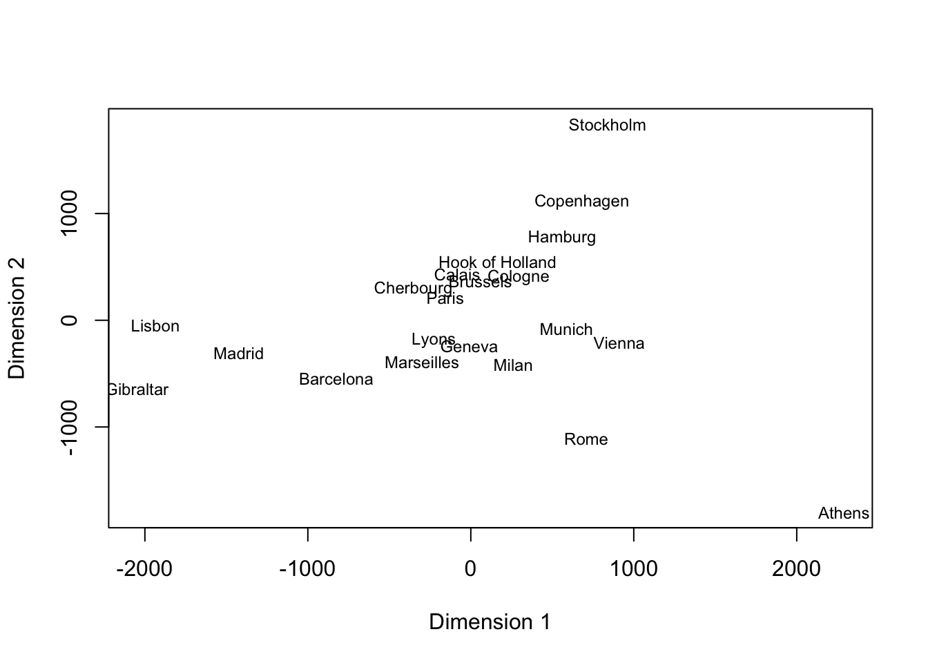
After applying a reflection of the map given by classical scaling to help it comply to the conventional orientation of a European map, the above plot reconstructs the European map quite well. Gibraltar, Lisbon and Madrid are in the south-west corner, the two North European cities Stockholm and Copenhagen are in the north end, and Athens is in the south-west corner.
Finally, let’s consider the 18 representative global cities. Their pairwise flight lengths (geodesic distance) are shown in the table below. As we can see, the geodesic distances between the three Southern-Hemisphere cities: Rio, Cape Town, Melbourne and other Northern-Hemisphere cities are generally large (almost all over 10,000 kilometers)
| Beijing | Cape Town | Hong Kong | Honolulu | London | Melbourne | Mexico City | Montreal | Moscow | New Delhi | New York | Paris | Rio | Rome | S.F. | Singapore | Stockholm | Tokyo | |
|---|---|---|---|---|---|---|---|---|---|---|---|---|---|---|---|---|---|---|
| Beijing | 0 | 12947 | 1972 | 8171 | 8160 | 9093 | 12478 | 10490 | 5809 | 2788 | 11012 | 8236 | 17325 | 8144 | 9524 | 4465 | 6725 | 2104 |
| Cape Town | 12947 | 0 | 11867 | 18562 | 9635 | 10388 | 13703 | 12744 | 10101 | 9284 | 12551 | 9307 | 6075 | 8417 | 16487 | 9671 | 10334 | 14737 |
| Hong Kong | 1972 | 11867 | 0 | 8945 | 9646 | 7392 | 14155 | 12462 | 7158 | 3770 | 12984 | 9650 | 17710 | 9300 | 11121 | 2575 | 8243 | 2893 |
| Honolulu | 8171 | 18562 | 8945 | 0 | 11653 | 8862 | 6098 | 7915 | 11342 | 11930 | 7996 | 11988 | 13343 | 12936 | 3857 | 10824 | 11059 | 6208 |
| London | 8160 | 9635 | 9646 | 11653 | 0 | 16902 | 8947 | 5240 | 2506 | 6724 | 5586 | 341 | 9254 | 1434 | 8640 | 10860 | 1436 | 9585 |
| Melbourne | 9093 | 10388 | 7392 | 8862 | 16902 | 0 | 13557 | 16730 | 14418 | 10192 | 16671 | 16793 | 13227 | 15987 | 12644 | 6050 | 15593 | 8159 |
| Mexico City | 12478 | 13703 | 14155 | 6098 | 8947 | 13557 | 0 | 3728 | 10740 | 14679 | 3362 | 9213 | 7669 | 10260 | 3038 | 16623 | 9603 | 11319 |
| Montreal | 10490 | 12744 | 12462 | 7915 | 5240 | 16730 | 3728 | 0 | 7077 | 11286 | 533 | 5522 | 8175 | 6601 | 4092 | 14816 | 5900 | 10409 |
| Moscow | 5809 | 10101 | 7158 | 11342 | 2506 | 14418 | 10740 | 7077 | 0 | 4349 | 7530 | 2492 | 11529 | 2378 | 9469 | 8426 | 1231 | 7502 |
| New Delhi | 2788 | 9284 | 3770 | 11930 | 6724 | 10192 | 14679 | 11286 | 4349 | 0 | 11779 | 6601 | 14080 | 5929 | 12380 | 4142 | 5579 | 5857 |
| New York | 11012 | 12551 | 12984 | 7996 | 5586 | 16671 | 3362 | 533 | 7530 | 11779 | 0 | 5851 | 7729 | 6907 | 4140 | 15349 | 6336 | 10870 |
| Paris | 8236 | 9307 | 9650 | 11988 | 341 | 16793 | 9213 | 5522 | 2492 | 6601 | 5851 | 0 | 9146 | 1108 | 8975 | 10743 | 1546 | 9738 |
| Rio | 17325 | 6075 | 17710 | 13343 | 9254 | 13227 | 7669 | 8175 | 11529 | 14080 | 7729 | 9146 | 0 | 9181 | 10647 | 15740 | 10682 | 18557 |
| Rome | 8144 | 8417 | 9300 | 12936 | 1434 | 15987 | 10260 | 6601 | 2378 | 5929 | 6907 | 1108 | 9181 | 0 | 10071 | 10030 | 1977 | 9881 |
| S.F. | 9524 | 16487 | 11121 | 3857 | 8640 | 12644 | 3038 | 4092 | 9469 | 12380 | 4140 | 8975 | 10647 | 10071 | 0 | 13598 | 8644 | 8284 |
| Singapore | 4465 | 9671 | 2575 | 10824 | 10860 | 6050 | 16623 | 14816 | 8426 | 4142 | 15349 | 10743 | 15740 | 10030 | 13598 | 0 | 9646 | 5317 |
| Stockholm | 6725 | 10334 | 8243 | 11059 | 1436 | 15593 | 9603 | 5900 | 1231 | 5579 | 6336 | 1546 | 10682 | 1977 | 8644 | 9646 | 0 | 8193 |
| Tokyo | 2104 | 14737 | 2893 | 6208 | 9585 | 8159 | 11319 | 10409 | 7502 | 5857 | 10870 | 9738 | 18557 | 9881 | 8284 | 5317 | 8193 | 0 |
The three-dimensional visualization result of classical MDS is shown above. You can rotate and magnify it on your laptop. The blue points represent Asian cities, the black points represent European cities, and the red points represent North American cities. If you inspect the plot clearly, you may notice that the cities appear to be constrained to the surface of a sphere, which complies to the true scenario.
In each of the examples, classical MDS was quite successful in generating maps which reflected the geographical configuration with continental or global maps which were (after some reflections/rotations) consistent with conventional maps. Let’s discuss the details.
4.4.1 Key features of MDS
MDS can be divided into three major types: Classical Scaling; Metric MDS; and Non-Metric MDS. The choice of method depends on the specifics of the distance/dissimilarity matrix and features which are preferential to preserve. Classical Scaling and Metric MDS require that the provided distances correspond to a metric (more on this below), while Non-metric MDS is usually used when the input data doesn’t satisfy the properties of a true distance metric or when the relationships are ordinal (i.e., we only know which distances are larger, but not by how much).
Beyond demonstrating the capacity of MDS to recover meaningful visualization, we also gain two insights from the examples above which hold for any MDS algorithm.
As we can tell from the recovery of US map and European map, the configurations of \(\tilde{y}_1, \tilde{y}_2, \dots, \tilde{y}_N\) are not unique, as we can rotate or flip the map. Actually, if \(\tilde{y}_1, \tilde{y}_2, \dots, \tilde{y}_N \in \mathbb{R}^{t^{\prime}}\) is considered as the optimal solution using Euclidean distance, then given any vector \(\vec{b} \in \mathbb{R}^{t^{\prime}}\) and orthogonal matrix \(A \in \mathbb{R}^{t^{\prime} \times t^{\prime}}\), \(||(A \tilde{y}_r + \vec{b} - (A \tilde{y}_s + \vec{b})|| = ||\tilde{y}_r - \tilde{y}_s||\). Rotation, Reflection or Translation don’t alter the pairwise distances. So \(A \tilde{y}_1 + \vec{b}, A \tilde{y}_2 + \vec{b}, \dots, A \tilde{y}_N + \vec{b}\) is also an optimal solution. Outside of Euclidean distances, reflections are still possible which eliminate the possibility of unique configurations.
The pairwise distance between two objects need not be Euclidean. In the above example, they are actually great circle distance.
In the following subsections, we will discuss the specifics of classical scaling with a brief discussion on two common methods of MDS, one each in metric and nonmetric MDS.
4.4.2 Classical Scaling
Let us first introduce some important definitions.
Definition 4.3 (Distance Matrix) A matrix \(\Delta \in \mathbb{R}^{N \times N}\) is called a distance matrix if it possesses the following properties:
Symmetry: \(\Delta\) is symmetric, meaning that: \(\Delta_{rs} = \Delta_{sr} \quad \text{for all } r \text{ and } s\)
Zero Diagonal: The diagonal entries of the matrix represent the distance of a point to itself, and are thus all zeros: \(\Delta_{rr} \equiv 0 \quad \text{for all } 1 \leq r \leq N\)
Non-negativity: All distances are non-negative: \(\Delta_{rs} \geq 0\)
Triangle Inequality: The distances in the matrix respect the triangle inequality: \[\Delta_{rs} \leq \Delta_{rt} + \Delta_{ts}\]
Distance matrices can be computed in many different ways. We will focus on the following specific case.
Definition 4.4 (Euclidean Distance Matrix) A distance matrix \(\Delta \in \mathbb{R}^{N \times N}\) is a Euclidean distance matrix if there exists a configuration \(\vec{y}_1, \vec{y}_2, \dots, \vec{y}_N\) s.t. \(\Delta_{rs}\) represents the Euclidean distance between points \(r\) and \(s\), i.e., \(||\vec{y}_r-\vec{y}_s||=\Delta_{rs} \forall r,s\).
Classical scaling operates under the assumption that \(\Delta\) is a Euclidean distance matrix though the dimensionality of the configuration \(\vec{y}_1,\dots,\vec{y}_N\) which gives rise to the distances specified by \(\Delta\) is unknown. As we shall see, the minimum dimensionality needed for the configuration to give the specified distances (assuming it exists at all) will be discovered through the classical scaling algorthm. Furthermore, since we are free to translate any configuration without altering pairwise distance, we will seek a configuration \(\vec{y}_1, \vec{y}_2, \dots, \vec{y}_N\) which is centered to simplify the following computation. The rotation of the configuration will also be given so that an optimal solution in \(k-1\) dimensions can be attained by dropping the final coordinate in the \(k\) dimensional configuration.
4.4.2.1 Recovering Coordinates
After some preprocessing, finding a centered configuration \(\vec{y}_1, \vec{y}_2, \dots, \vec{y}_N\) from the Euclidean distance matrix \(\Delta\) is possible through some of the linear algebra techniques we have discussed so far. Observe that \(\Delta^2_{rs}\) can be expressed as \[\Delta^2_{rs} = ||\vec{y}_r||^2 + ||\vec{y}_s||^2 - 2 \vec{y}_r^T \vec{y}_s\] so that \[\vec{y}_r^T\vec{y}_s = -\frac{1}{2}\left(\Delta_{rs} - \|\vec{y}_r\|^2 - \|\vec{y}_s\|^2 \right).\] We will use this relationship to build an inner product matrix \({\bf B}\) with entries \({\bf B}_{rs} = \vec{y}_r^T\vec{y}_s\). In matrix form, we may write \[{\bf B} = {\bf Y Y}^T\], where \({\bf Y}\) is a data matrix containing the configuration \(\vec{y}_1,\dots,\vec{y}_N\) with Euclidean distances \(\Delta\).
1) Computing the inner product matrix \(B\)
The inner product term can be represented as: \(B_{ij} = \vec{y}_i^T \vec{y}_j\). As a result, \[(\Delta_{ij})^2 = B_{ii} + B_{jj} - 2 B_{ij}.\]
Key Observation In the previous line, we express the entries of \(\Delta\) (known) with entries of \(B\) (unknown). Our goal is to find a way to express entries of \(B\) (unknown) with entries of \(\Delta\). Intuitively, we want to cancel out \(B_{ij}\) terms in the expression. Considering that \(\sum_{i=1}^N \vec{y}_i = \vec{0}\), we sum both sides of the equation over the index \(i\). We can get the following expression:
\[\sum_{i=1}^N (\Delta_{ij})^2=\operatorname{tr}(B) + N B_{ii}\]
Similarly, we can also sum both sides of the equation over index \(j\), and get the expression: \[\sum_{j=1}^N (\Delta_{ij})^2=\operatorname{tr}(B) + N B_{jj}\]
We successfully eliminate all the off-diagonal terms of \(B\) through the above steps. Now, we want to take a step further. Sum both sides of the equations over both indexes \(i\) and \(j\). We acquire the following expression: \[\sum_{i=1}^N \sum_{j=1}^N (\Delta_{ij})^2 = 2N \operatorname{tr}(B)\]
Now we can solve the entries of \(\Delta\) using the entries of \(B\) through a backward calculation. From the last equation, we get \[\operatorname{tr}(B) = \frac{1}{2N} \sum_{i=1}^N \sum_{j=1}^N \Delta_{ij}^2\]
Then substitute the above expression into above formulas, we get the expression of the diagonal entries of \(B\):
\[B_{ii} = \frac{1}{N} (\sum_{j=1}^{N} (\Delta_{ij})^2 - \operatorname{tr} (B))\]
After that, we can finally get the off-diagonal entries of \(B\):
\[\begin{align*} B_{ij} & = \frac{1}{2} (B_{ii} + B_{jj} - (\Delta_{ij})^2) \\ & = -\frac{1}{2} (\Delta_{ij})^2 + \frac{1}{N} \sum_{i=1}^N (\Delta_{ij})^2 + \frac{1}{N} \sum_{j=1}^N (\Delta_{ij})^2-\frac{1}{2 N^2} \sum_{i=1}^N \sum_{j=1}^N (\Delta_{ij})^2 \end{align*}\]
We may more compactly express the inner product matrix \(B\) in a matrix form, as \[B = HAH\] where \(A \in \mathbb{R}^{N \times N}\) has entries \(A_{ij} = -\frac{1}{2}(\Delta_{ij}) \quad \text{for} \; \forall \; 1 \leq i,j \leq N\) and \(H\) is the centering matrix \[H = \mathbb{I}_N - \frac{1}{N} \mathbb{1}_N \mathbb{1}_N^T\].
2) Recover the coordinates using inner product matrix \(B\)
Both diagonal and off-diagonal entries of the inner product matrix \(B\) has been shown. We assumed that \(B\) = \(YY^T\), so \(B\) is symmetric and positive semi-definite (all eigenvalues are non-negative). Assuming \(B\) is rank \(t\) implies that it has \(t\) positive eigenvalues and \(N-t\) ‘zero’ eigenvalues.
Our intuition is to apply SVD/diagonalization to \(B\) in order to recover the configuration \(\vec{y}_1, \vec{y}_2, \dots, \vec{y}_N \in \mathbb{R}^t\) by computing the nonzero eigenvalues and corresponding eigenvectors giving the factorization.
\[\begin{align*} B & = \left(\vec{u}_1\left|\vec{u}_2\right| \ldots \mid \vec{u}_t\right) \begin{pmatrix} \lambda_1 & \cdots & 0 \\ \vdots & \ddots & \vdots \\ 0 & \cdots & \lambda_t \end{pmatrix} \left(\begin{array}{c} \vec{u}_1^{\top} \\ \vec{u}_2^{\top} \\ \vdots \\ \vec{u}_t^{\top} \end{array}\right) \\ & = \tilde{U} \begin{pmatrix} \lambda^{1/2}_1 & \cdots & 0 \\ \vdots & \ddots & \vdots \\ 0 & \cdots & \lambda^{1/2}_t \end{pmatrix} \begin{pmatrix} \lambda^{1/2}_1 & \cdots & 0 \\ \vdots & \ddots & \vdots \\ 0 & \cdots & \lambda^{1/2}_t \end{pmatrix} \tilde{U}^T \\ & = (\tilde{U} \Lambda^{1/2}) (\tilde{U} \Lambda^{1/2})^T \end{align*}\]
Let \(Y=\tilde{U} \Lambda^{1/2}\), so that rows of \(\tilde{U} \Lambda^{1/2}\) correspond to the vectors \(\vec{y}_1, \vec{y}_2, \dots, \vec{y}_N\). It satisfies every entry of the inner product matrix \(B\), as well as all pairwise distances \(\Delta_{ij}\)! Importantly, the rank of \(B\) immediately indicates the minimal dimension needed to recover a configuration which exactly recovers the Euclidean distances in \(\Delta.\)
For visualization, we may prefer a lower dimensional configuration than the dimensionality \(t\) discovered through classical scaling. For a \(k < t\) dimensional configuration, we instead use the first \(k\) columns of \(\tilde{U}\Lambda^{1/2}\) as a our \(k\)-dimensional vectors. Outside of optimal recovery, we may instead formulate the classical scaling problem in \(k\)-dimensions as the following minimization problem.
\[\text{argmin}_{Y \in \mathbb{R}^{N\times k}} \| B - YY^T\|_F\] from which it follows that \(YY^T\) is built from the rank \(k\) approximation to \(B\). Using the results from SVD and the equivalence of SVD and eigendecompositions for symmetric positive, semidefinite matrices, this is equivalent to using the first \(k\) columns of \(\tilde{U}\Lambda^{1/2}\).
Dealing with real data case
For a given distance matrix, the Euclidean condition may not hold. In the previous globe map example, the distance matrix is based on the geodesic distance instead of the Euclidean distance. Under this circumstance, the “inner product” matrix \(B = HAH\) is still symmetric but will not be positive definite. As a simpler example, consider the following case
Example 4.4 (Non Euclidean Distances) Suppose we have a distance matrix \(\Delta\):
Given the matrix: \[ \Delta = \begin{pmatrix} 0 & 1 & 1 & 2 \\ 1 & 0 & 1 & 1 \\ 1 & 1 & 0 & 1 \\ 2 & 1 & 1& 0 \end{pmatrix} \]
##      [,1] [,2] [,3] [,4]
## [1,]    0    1    1    2
## [2,]    1    1    0    1
## [3,]    1    1    0    1
## [4,] 2 1 1 0- Compute matrix \(A\) as: \[ A = -\frac{1}{2} \Delta^2 \]
##      [,1] [,2] [,3] [,4]
## [1,]  0.0 -0.5 -0.5 -2.0
## [2,] -0.5 -0.5  0.0 -0.5
## [3,] -0.5 -0.5  0.0 -0.5
## [4,] -2.0 -0.5 -0.5 0.0- Compute matrix \(B\) using: \[ H = I - \frac{1}{n} \mathbf{11}^T \] Where \(I\) is the identity matrix and \(n\) is the number of rows (or columns) in \(\Delta\). Then: \[ B = H A H \]
##         [,1]    [,2]    [,3]    [,4]
## [1,]  0.9375  0.1875 -0.0625 -1.0625
## [2,]  0.0625 -0.1875  0.0625  0.0625
## [3,]  0.0625 -0.1875  0.0625  0.0625
## [4,] -1.0625 0.1875 -0.0625 0.9375- Finally, perform an eigen-decomposition on matrix \(B\) which gives eigenvalues.
## [1] 2.00 -0.25 0.00 0.00Here, we have a negative eigenvalue \(-\frac{1}{4}\). This indicates the original distance matrix \(\Delta\) is not a Euclidean distance matrix; there is no Euclidean space containing four vectors with the given pairwise distances!!
Other practical issues
Asymmetric \(\Delta\): There are cases where the distance matrix \(\Delta\) is not symmetric. In this case, we usually set \(\Delta \leftarrow \frac{1}{2}(\Delta + \Delta^T)\) to enforce symmetry.
When there exist some negative eigenvalues in the inner product matrix \(B\), we usually have two options to deal with it.
Inflate the original proximity matrix \(\Delta\) by a small constant factor \(c\), i.e., \(\Delta_{ij} \leftarrow \Delta_{ij} + c, \; \text{if} \; i \neq j\) until \(B\) is positive semidefinite.
If there exist several negative eigenvalues with small absolute value (compared to the largest several positive eigenvalues), and there are more positive eigenvalues than our prior estimation (the dimension of the original configuration), we may just pick the largest \(t\) eigenvalues and eliminate the rest.
Example 4.5 (Global Cities Revisited) We can also consider the previous global city distance matrix example. Plot the scree plot of the inner product matrix.
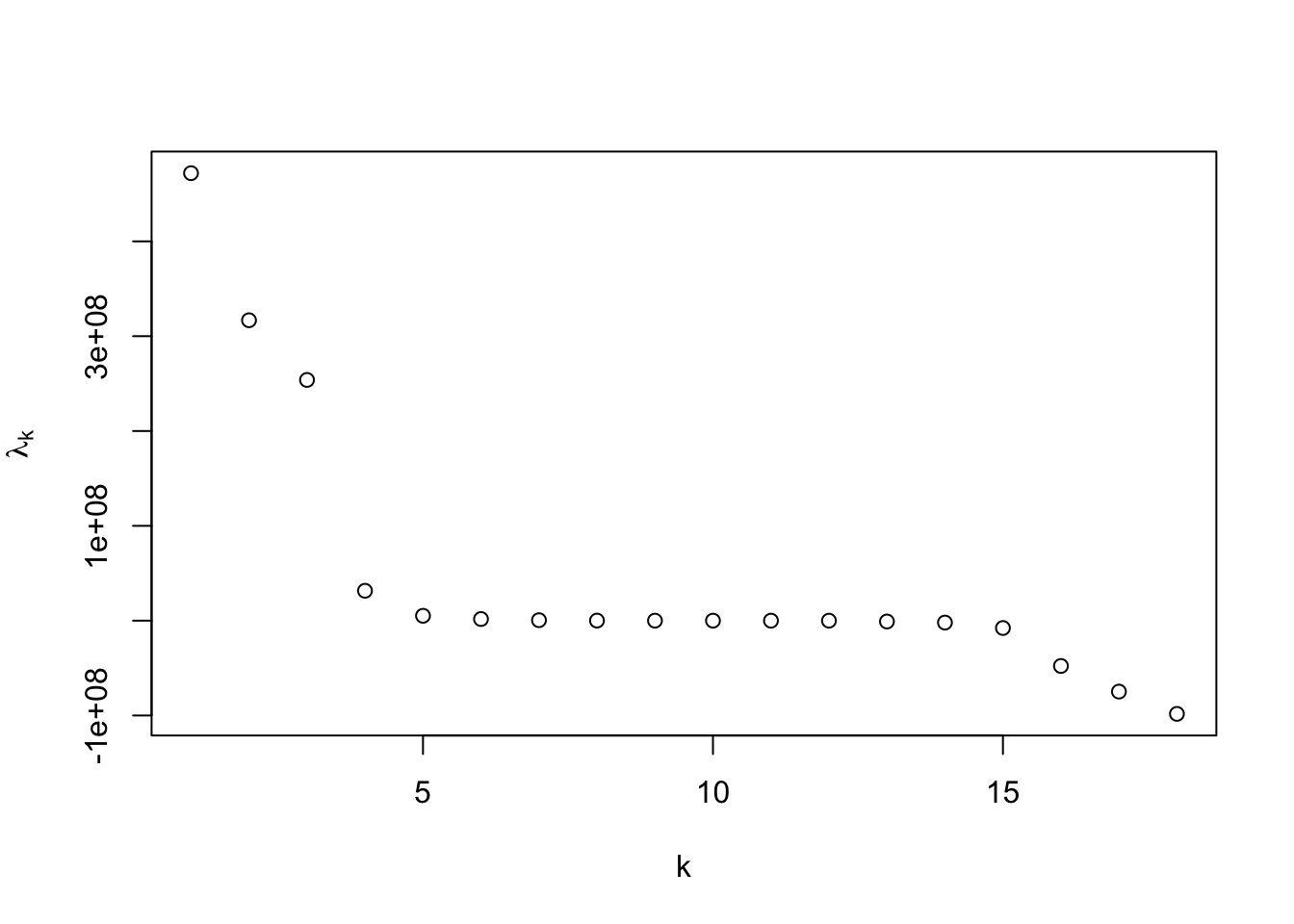
We find that the first three eigenvalues are much larger than the rest, so we assume that the dimension of the original configuration is 3, which also complies to our knowledge about global map.
4.4.2.2 Duality of PCA and Classical Scaling
“There is a duality between a principals components analysis and classical MDS where dissimilarities are given by Euclidean distance”[17].
Given the matrix expression of the original configuration \(\mathbf{X} \in \mathbb{R}^{N \times d}\). Recall that PCA is attained by finding the eigen-vectors of the covariance matrix \(\frac{1}{N-1} (HX)^T (HX)\), where \(H\) is the centering matrix. Suppose the \(k\) eigen-vectors are \(\vec{w}_1, \vec{w}_2, \dots, \vec{w}_k\), and the corresponding eigenvalues are \(\mu_1, \mu_2, \dots,\mu_k\). Then \(HX=YW^T\), where \(W=(\vec{w}_1 | \vec{w}_2 | \dots | \vec{w}_N)\) represents PC Loadings, and \(Y\) represents PC Scores.
While MDS is attained by first converting \(X\) into distance matrix, here, Euclidean distance. In the classical MDS algorithm, the process of converting the Euclidean distance matrix into the inner product matrix gives \(B=(HX)(HX)^T\). then we find the eigenvectors of \(B\) which are equivalent to the left singular vectors of \(HX\) and with nonzero eigenvalues \(\lambda_1, \lambda_2, \dots, \lambda_d\) which are the squared singular values of \(HX\).
Recall what you have learned in Linear Algebra. The eigenvalues of \(HX(HX)^T\) are the same as those for \(X^TX\), together with an extra n-p zero eigenvalues. So the first \(t\) PC scores give the t-dimensional configuration for Classical Scaling. Choosing the number of dimensionality \(t\) of the original configuration is equivalent to choosing the number of principal components to keep.
Furthermore, we have shown that \(HX=YW^T\), then \(B=(HX)(HX)^T=YW^TWY^T=YY^T\), this means PC scores are the exact solutions for Classical Scaling! As a result, classical MDS has the same strengths and weaknesses of PCA.
4.4.3 Metric MDS
Metric MDS is a set of algorithms which seek optimal configuration which minimize a specified loss function. Typically, this loss function is called the stress which has the general form \[S(\vec{y}_1,\dots,\vec{y}_N) = \sum_{i < j} W_{ij} \left(\|\vec{y}_i-\vec{y}_j\|^2 - \Delta_{ij}\right)^2 = \frac{1}{2}\sum_{i\ne j} W_{ij}\left(\|\vec{y}_i-\vec{y}_j\|^2 - \Delta_{ij}\right)^2\] where the weights \(W_{ij}\ge 0\) have different conventions which prioritize the preservation of certain distances in the original coordinates. Heuristically, you can think of \(\left(\|\vec{y}_i-\vec{y}_j\|^2 - \Delta_{ij}\right)^2\) as measuring how far the lower-dimensional Euclidean distances \(\|\vec{y}_i-\vec{y}_j\|\) deviate from the specified original distance \(\Delta_{ij}\). Importantly, there is no closed form expression for \(\vec{y}_1,\dots,\vec{y}_N\) which minimize \(S\) so gradient based optimization methods are typically used in practice. When the desired dimension is unknown, one can estimate different \(\vec{y}_1,\dots,\vec{y}_N\) in different dimensions and compare the optimal stress as a data driven method for choosing the dimensionality.
A important method of metric MDS is the Sammon mapping which takes \(W_{ij} \propto \frac{1}{\Delta_{ij}}\). Thus, if \(\Delta_{ij} \gg \Delta_{k\ell}\) it follows that \(W_{ij} \ll W_{k\ell}\) and we may infer that the Sammon mapping places a greater emphasis on the preservation of small distances! Briefly, we show the results of the Sammon mapping applied to the global cities data.
Example 4.6 (Sammon mapping and global cities) First, we show the minimal Sammon stress at each dimension.
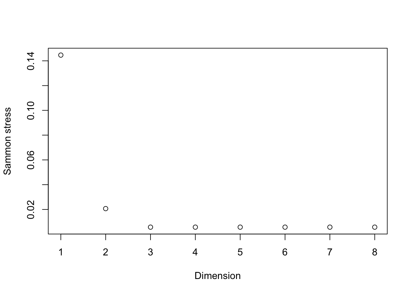
Figure 4.9: Sammon stress for Global Cities Data
## A marker object has been specified, but markers is not in the mode
## Adding markers to the mode...
This stress saturates near a small value for dimensions three and up suggesting a three dimensional configuration is suitable. We show this result below. Note its similarities to the result of classical scaling (which is default initialization for the Sammon mapping optimization algorithm).
4.5 Exercises
Show that the PCA scores are centered.
Suppose a data matrix \({\bf X}\in\mathbb{R}^{N\times d}\) has principal component scores \({\bf Y}\in\mathbb{R}^{N\times d}\), principal component loading matrix \({\bf W}\in\mathbb{R}^{d\times d}\), and principal component variances \(\lambda_1,\dots,\lambda_d\). Show that the sample covariance of the PCA scores, \({\bf Y}\), is diagonal.
Consider the data matrix \[{\bf X} = \begin{bmatrix} 2 & 3 \\ 4 & 5\\ 6& 7 \\ 8 & 9 \end{bmatrix}.\]
- Compute the principal component scores, variances, and loadings of \({\bf X}.\)
- Does \({\bf X}\) exhibit lower dimensional structure? If so, describe it.
Given a dataset with outliers: \[ \mathbf{X} = \begin{bmatrix} 1 & 2 \\ 2 & 4 \\ 3 & 6 \\ 4 & 8 \\ 100 & 200 \end{bmatrix} \]
- Center the data.
- Compute the covariance matrix.
- Perform PCA and identify the principal component scores, loadings, and variances.
- Discuss how outliers affect PCA and suggest ways to handle them.
Consider a dataset: \[ \mathbf{X} = \begin{bmatrix} 1 & 100 \\ 2 & 200 \\ 3 & 300 \\ 4 & 400 \end{bmatrix} \]
- Center the data.
- Compute the covariance matrix.
- Perform PCA and find the principal components.
- Discuss the importance of feature scaling in PCA.
Given a nonlinear dataset: \[\mathbf{X} = \begin{bmatrix} 1 & 1 \\ 2 & 4 \\ 3 & 9 \\ 4 & 16 \\ 5 & 25 \end{bmatrix}\]
- Center the data.
- Compute the covariance matrix.
- Perform PCA and identify the principal components.
- Discuss the limitations of PCA for nonlinear datasets and suggest alternative methods.
Load the Iris dataset and standardize the features.
- Perform PCA on the standardized data.
- Plot the cumulative explained variance as a function of the number of principal components.
- Choose the number of principal components that explain at least 95% of the variance.
- Project the data onto the chosen principal components and visualize the results.
- Discuss the results and the effectiveness of PCA in reducing the dimensionality of the dataset.
Suppose \[\vec{x}=(x_1,x_2)^T \sim \mathcal{N}\left(\begin{bmatrix} 0\\ 0\end{bmatrix}, \begin{bmatrix}1 & \rho \\ \rho & 1\end{bmatrix}\right),\] i.e. random vector \(\vec{x}\) follows a multivariate normal distribution with mean \(\vec{0}\) and covariance \(\Sigma_X = \begin{bmatrix}1 & \rho \\ \rho & 1\end{bmatrix}\). Let \(w = \frac{\sqrt{2}}{2}(x_1+x_2)\) and \(z = \frac{\sqrt{2}}{2}(x_1-x_2).\) Find the joint distribution of \((w,z)^T\). Hint: linear combinations of normal random variables are also normal.
Consider a data matrix \(X \in \mathbb{R}^{N\times d}\) with centered columns so that the sample covariance matrix is \[\hat{\Sigma} = \frac{X^TX}{N}.\] Assume \(\hat{\Sigma}\) has eigenvalues \(\lambda_1 > \lambda_2 >\dots > \lambda_d >0\) with orthonormal eigenvectors \(\vec{w_1},\dots,\vec{w}_d.\)
If \(X^{(1)} = X - X\vec{w}_1\vec{w}_1^T\) is the data matrix where each row has had its component in the direction of \(\vec{w}_1\) removed, show that \[\hat{\Sigma}^{(1)} = \frac{{X^{(1)}}^T X^{(1)}}{N} = \hat{\Sigma} - \lambda_1 \vec{w}_1\vec{w}_1^T.\]
Show that \(\hat{\Sigma}\) can be written in the form \(\hat{\Sigma} = \sum_{j=1}^d \lambda_j \vec{w}_j\vec{w}_j^T.\)
For \(k < d\), let \(\vec{q}_1,\dots,\vec{q}_k\in\mathbb{R}^d\) be fixed orthonormal vectors. Suppose \(a_1,\dots,a_k\) are independent Gaussian random variables with mean zero and variances \(\lambda_1>\dots>\lambda_k\) respectively. Let \[\vec{x} = a_1\vec{q}_1+\dots+a_k+\vec{q}_k + \vec{\epsilon}\] where \(\vec{\epsilon}\sim\mathcal{N}(\vec{0},\sigma^2{\bf I})\) is independent of \(a_1,\dots,a_k\)
- Find the mean and covariance of \({\bf X}\).
- Find the eigenvalues and eigenvectors of \({\bf \Sigma}\).
- For \(d = 10\) and $k=3 and let \(\lambda_1 = 25,\, \lambda_2 = 9,\,\lambda_3 = 4\) and \(\sigma^2=1\). Generate 100 independent realizations of \(\vec{x}\) and compute the principal component loadings and variances. How do these compare to your results from b.
- Repeat c. for \(10^4\) samples. How have the results changed?
Let \(\vec{x}_1,\dots,\vec{x}_N\) be vectors in \(\mathbb{R}^d\). Assume a PCA of these data has loadings \(\vec{w}_1,\dots,\vec{w}_d\) with associated variances \(\lambda_1 \ge \dots \ge \lambda_d \ge 0.\) Let \(U\) be a \(d\times d\) orthonormal matrix and set \(\vec{y}_i = U\vec{x}_i.\) Find expressions for the principal component loadings and variance of \(\vec{y}_1,\dots,\vec{y}_N\) in terms of \(U\), \(\vec{w}_1,\dots,\vec{w}_d\) and \(\lambda_1,\dots,\lambda_d.\)
Load the mtcar dataset containing 11 observations from 32 cars.
Show the principal component loadings and a biplot of the first and second PC components.
Rescale the mpg (miles per gallon) data to feet per gallon, i.e. mtcars$mpg <- 5280mtcars$mpg.* Rerun PCA on these modified data and show the loadings and biplot.
What is the first loading capturing? Explain this result.
Rerun the results using the empirical correlation matrix by setting the option scale = TRUE in the prcomp command. Compare this result with part (a)
Consider the helix data shown below from two different directions.

Figure 4.10: Helix data
What is the dimension of the shape formed by these data?
Compute the three principal component variances and show them below.
Do the principal component variances reflect the dimension of the data? Why or why not?
Consider a dataset with three features: \[\mathbf{X} = \begin{bmatrix} 2 & 0 & 1 \\ 3 & 2 & 2 \\ 4 & 4 & 3 \\ 5 & 6 & 4 \\ 6 & 8 & 5 \end{bmatrix}\]
- Center the data by subtracting the mean of each feature.
- Compute the covariance matrix of the centered data.
- Find the eigenvalues and eigenvectors of the covariance matrix.
- Project the data onto the first two principal components.
- Visualize the original data and the projected data in a 2D plot.
- Discuss how PCA can help in reducing the dimensionality of the data while preserving important information.
The dataset simplex10 contains samples generated from the probability simplex in \(\mathbb{R}^{10}\). (This means all entries nonnegative and each random vector has entries which sum to one.)
Run PCA, SVD, and NMF on these data and compare the results. In particular, what lower dimensional structure, if any, do these methods indicate?
Why do the results differ?
Show that the Frobenius norm of a matrix is the square of the sum of its squared singular values. You may use the helpful identity \(\|{\bf A}\|_F^2 = tr({\bf AA}^T)\)